

Abstract
The impact of the Atlantic water inflow (AW inflow) into the Barents Sea on the regional cyclone activity in winter is analyzed in 10 ensemble simulations with the coupled Arctic atmosphere-ocean-sea ice model HIRHAM-NAOSIM for the 1979–2016 period. The model shows a statistically robust connection between AW inflow and climate variability in the Barents Sea. The analysis reveals that anomalously high AW inflow leads to changes in static stability and wind shear in the lower troposphere, and thus favorable conditions for cyclogenesis in the Barents/Kara Seas. The frequency of occurrence of cyclones, but particularly of intense cyclones, is increased over the Barents Sea. Furthermore, the cyclones in the Barents Sea become larger (increased radius) and stronger (increased intensity) in response to an increased AW inflow into the Barents Sea, compared to years of anomalously low AW inflow.
Export citation and abstract BibTeX RIS

Original content from this work may be used under the terms of the Creative Commons Attribution 4.0 licence. Any further distribution of this work must maintain attribution to the author(s) and the title of the work, journal citation and DOI.
1. Introduction
The Barents Sea is a key Arctic region, because much of both atmospheric and oceanic heat transports into the Arctic occurs over there. Along with Fram Strait, the Barents Sea Opening (BSO) is a gateway for Atlantic water (AW) inflow of warm and salty water toward the Arctic Ocean. The AW inflow accounts for the partly ice-free Barents Sea during winter. Current warm climate conditions are characterized by increased Atlantic northward ocean heat transport (strengthening and warming of the inflow) to the Barents Sea, reduced Arctic sea ice cover and high air temperatures (Årthun et al 2012, Smedsrud et al 2013, Muilwijk et al 2018, van der Linden et al 2019). Increased AW inflow into the Barents Sea results in a warming and salinification, which may lead to 'Atlantification' of the Barents Sea (Polyakov et al 2017, Barton et al 2018, Årthun et al 2019). According to Lind et al (2018), a sharp increase in ocean temperature and salinity is apparent from the mid-2000s onwards and can be linked to recent decline in sea ice import and corresponding loss in freshwater, leading to weakened ocean stratification, enhanced vertical mixing and increased upward fluxes of heat and salt that prevent sea ice formation. The connection between AW inflow and sea ice allows to predict the winter Arctic sea ice cover on different time scales (Nakanowatari et al 2014, Yeager et al 2015, Årthun et al 2017).
On the other hand, variations in the oceanic inflow into the Barents Sea play also a crucial role for the atmospheric conditions. Variability in the inflow is related with surface air temperature variability (on a time scale of a few years or more) in the Arctic region during the winter season (e.g. Semenov 2008, Schlichtholz 2011, 2019, Smedsrud et al 2013, Ivanov et al 2016). Furthermore, the increased AW inflow and the corresponding sea ice retreat in winter leads to enhanced turbulent heat loss to the atmosphere and a regional cyclonic circulation anomaly that may lead to further increasing inflow, suggesting a positive feedback (Ådlandsvik and Loeng 1991, Bengtsson et al 2004). This may enhance regional climate variations and result in rapid regional climate changes (Semenov et al 2008, Mokhov et al 2009, Chernokulsky et al 2017).
Interactions between AW inflow and the associated changes in the oceanic and atmospheric conditions in the Barents Sea occur on time scales from one month (e.g. Sandø et al 2010, Lien et al 2017) to one year (e.g. Årthun et al 2012, Onarheim et al 2015). Smedsrud et al (2013) sketch two feedback loops associated with the Atlantic heat transport and which involve coupled atmosphere-ice-ocean variability (their figure 3).
Inoue et al (2012) showed that the sea ice variability in the Barents Sea very likely controls the cyclone tracks in that region through changes in baroclinicity. A statistical connection between Arctic sea ice changes and cyclone activity over the Arctic Ocean has been reported (Koyama et al 2017, Wei et al 2017). Koyama et al (2017) found that an increase in moisture availability and regional baroclinicity as well as changes in vertical stability due to reduced sea ice in September favor cyclogenesis. The increase of open water areas in the Arctic have led to increased fluxes of heat and moisture from the ocean to the atmosphere, warming and moistening the Arctic atmosphere and increasing the potential for cyclogenesis, in particular for polar lows (e.g. Kolstad et al 2016). A relationship between polar low genesis/intensification and decreasing sea ice cover and increasing sea surface temperature (SST) in the Norwegian and Barents Seas was found (Kolstad and Bracegirdle 2017, Sergeev et al 2018)
Cyclones, in turn, can affect AW inflow, sea ice reduction through wind forcing of ice motion and divergence, and indirectly through advection of heat and moisture, changed radiative balance and cloud feedbacks, and modified energy fluxes (e.g. Zhang et al 2012, Parkinson and Comiso 2013, Boisvert et al 2016, Sun and Gao 2018, Semenov et al 2019). Warming and sea ice decline in the Atlantic sector of the Arctic Ocean result in a larger open water area, which serves as a source of heat and moisture during the long cold season when the atmosphere quickly becomes significantly colder than the ocean surface (e.g. Alexeev et al 2017).
This study analyzes changes in winter cyclone activity associated with the variability of AW inflow into the Barents Sea. Particularly, we examine the role of anomalously high AW inflow for changes of the cyclone activity characteristics and their related atmospheric conditions in the Barents Sea. The study focuses on the winter (December–February) for the 1979–2016 period. We extend previous studies by the following novel and important aspects: (i) we detailed analyze the lower-troposphere baroclinicity with the measure of the Eady growth rate (EGR) and their two contributing factors, namely the atmospheric static stability and wind shear; (ii) we present the impact of AW inflow on the three main cyclone characteristics, namely the cyclone frequency, depth, and size. Further, we look separately on the frequency of occurrence of intense and non-intense cyclones; (iii) our analysis is based on ensemble simulations of a coupled Arctic atmosphere-ocean-sea ice regional climate model (RCM). The RCM allows a relatively high spatial resolution (in our case ca. 27 km in the atmosphere and ca. 9 km in the ocean), which enables a better representation of mesoscale atmospheric processes, important for cyclone activity. Furthermore, a coupled model includes the atmosphere-ocean interaction, which often occurs at high spatiotemporal scales. The ensemble approach allows to analyze different realizations of possible climate states, whereby random correlations can be excluded. The linkage between AW inflow and climate variability in the Barents Sea, particularly in terms of cyclogenetic factors, can therefore, be rated as process-based linkage.
2. Data and methods
2.1. Model data
In the present study, we use data from simulations with the most recent version of the coupled Arctic RCM HIRHAM-NAOSIM (Dorn et al 2019). This version consists of the atmosphere component HIRHAM5, which is set up for a domain that covers the whole Arctic north of about 60° N using a rotated spherical coordinate system with horizontal resolution of 0.25° (approximately 27 km). In the vertical, HIRHAM5 comprises 40 levels from about 10 m above the surface up to a pressure level of 10 hPa, with the highest vertical resolution in the lower troposphere. The ocean-sea ice component NAOSIM (North Atlantic/Arctic Ocean Sea-Ice Model) is based on the Geophysical Fluid Dynamics Laboratory Modular Ocean Model MOM-2 (Pacanowski 1996) and the dynamic-thermodynamic sea ice model described by Harder et al (1998) with substantial modifications of the ice thermodynamics introduced by Dorn et al (2009). NAOSIM is set up for a domain that encloses the entire Arctic Ocean, the Nordic seas, and the northern North Atlantic (with the southern model boundary at approximately 50° N) using a rotated spherical coordinate system with horizontal resolution of 1/12° (approximately 9 km). NAOSIM comprises 50 vertical levels at the maximum (depending on the ocean depth) with vertical resolution of 10 m in the upper ocean.
An ensemble of 10 hindcast simulations was carried out for the period 1979–2016. The RCM simulations were driven by ERA-Interim reanalysis data (Dee et al 2011) at the lateral atmospheric boundaries and all surface boundaries outside the coupling domain. The latter particularly plays a role for the NAOSIM domain which extends further to the south in the Atlantic sector than the HIRHAM domain. At NAOSIM's lateral boundary in the northern North Atlantic, an open-boundary condition is implemented following the formulation of Stevens (1991). At inflow points, temperature and salinity are restored to the Levitus climatology (Levitus and Boyer 1994, Levitus et al 1994) with a time constant of 30 d. The individual ensemble members only differ in their initial conditions for the ocean and the sea ice at the very beginning of the simulations in January 1979. For this purpose, initial ocean and sea ice fields were taken from the Januaries 1991–2000 of a preceding coupled spin-up run for the period 1979–2000. A detailed description of both the model and the ensemble simulations is given by Dorn et al (2019).
Our study region is the Barents Sea (65°–85° N, 20°−60° E) (red box in figure 1(a)). Analyses are performed for the winter (here defined as the period from December to February) 1979–2016. We use 6-hourly mean sea level pressure (MSLP) for cyclone identification (section 2.2), 6-hourly data for the EGR calculation (section 2.3), and monthly mean data of near-surface air temperature, sea ice concentration, sea ice thickness, MSLP, surface (sensible and latent) turbulent heat fluxes, ocean temperature and current velocity for the composite analysis (section 2.4). The AW inflow for the BSO is computed for the model water column down to a depth of 337 m. This is appropriate since the AW core is predominantly located at less than 300 m depth (e.g. Skagseth 2008).

Figure 1. Composite difference 'High minus low AW inflow in winter' for (a) sea ice concentration, (b) sea ice thickness (m), (c) surface air temperature (K; color shading) and total (latent+sensible) surface turbulent heat flux (W m−2; isolines), (d) sea level pressure (hPa; color shading) and geopotential height at 250 hPa (gpm; isolines) for winter (DJF). The line labeled with BSO in (a) indicates the Barents Sea Opening. Black dots indicate statistical significance (p < 0.05) for the differences presented by color shading. Yellow and green isolines show positive and negative changes. For the heat flux changes only isolines for ±5 and ±10 W m−2 are included.
Download figure:
Standard image High-resolution image2.2. Cyclone identification
An algorithm of cyclone identification (Bardin and Polonsky 2005, Akperov et al 2007, Akperov et al 2015) is applied on 6-hourly MSLP data from the ensemble simulations. The algorithm is based on minima in the MSLP fields and has been applied in several other studies that investigated changes in cyclone activity in extratropical and high latitudes (Neu et al 2013, Ulbrich et al 2013, Simmonds and Rudeva 2014, Akperov et al 2018), including polar mesocyclones (Akperov et al 2017). Cyclone frequency, depth, and size are analyzed. The cyclone frequency is defined as the number of cyclone events per season. We consider the cyclone depth as a measure of cyclone intensity. The cyclone depth is determined as the difference between the minimum central pressure in the cyclone and the outermost closed isobar. As shown in previous studies (e.g. Golitsyn et al 2007, Simmonds and Keay 2009), the depth provides a direct measure of the kinetic energy of the system. Deep (intense) cyclones are identified by anomalously strong depth exceeding the 95th percentile of the cyclone depth distribution from the simulations; i.e. cyclones with depths exceeding 20 hPa are considered (Zahn et al 2018). The cyclone size (radius) is determined as the average distance from the geometric center to the outermost closed isobar. To map spatial patterns of cyclone characteristics we use a grid with circular cells of a 2.5° latitude radius. The cyclone identification algorithm is described in detail in appendix.
2.3. Measure of baroclinic instability
Baroclinic instability contributes to formation, intensification and persistence of cyclones in the atmosphere. A simple parameter measuring the low-level baroclinic instability is the EGR (e.g. Lindzen and Farrell 1980, Hoskins and Valdes 1990). This parameter involves the vertical wind shear and the Brunt–Väisälä frequency:

where f is the Coriolis parameter, N is the Brunt–Väisälä frequency, V is the horizontal wind speed, and z is the height. The Brunt–Väisälä frequency, which is a measure of atmospheric static stability, is given by:

where g is the gravity acceleration and θ is the potential temperature. For the calculation of EGR, we use 6-hourly data for wind, temperature, and geopotential height for two levels in the lower atmosphere (500 and 850 hPa). Those vertical levels have been chosen to cover the lower half of the tropospheric column but above the planetary boundary layer which top is typically around the 850 hPa level.
2.4. Compositing of AW inflow
The AW inflow for the BSO is computed for the model water column down to a depth of 337 m (whereas the depth of the most part of the Barents Sea is less than 300 m) as  where A represents the BSO (area between Svalbard and Norway; see figure 1(a)). v is the ocean current normal to the area, which is positive (negative) if water flows into (out of) the Barents Sea (Long and Perrie 2017). The associated ocean heat transport is calculated as
  where ρ and Cp are constant density and specific heat, T is the ocean temperature and T0 is the reference temperature, which is set to 0 °C as commonly used in the oceanographic community. This value is representative for the cold waters leaving the Barents Sea.
Using the calculated time series of the simulated AW inflow for the BSO, low and high AW inflow years with respect to the winter (December–February) were selected for each ensemble member. Low and high AW inflow cases were selected when the deviation of the AW inflow from the ensemble mean was larger than one standard deviation. These cases were combined into composite means, and composite differences ('low minus high AW inflow') for atmospheric and oceanic variables. In total, the composite analysis comprises 37 cases for low and high AW inflow conditions.
The statistical significance of the calculated differences in atmospheric and oceanic variables and cyclone activity characteristics was estimated using Student's t-test with 95% confidence level. The temporal correlation analysis is based upon the Pearson correlation coefficient (R).
3. Impact of anomalously high AW inflow on sea ice and atmosphere
3.1. AW inflow
Before investigating the response of cyclone activity to AW inflow changes, it is informative to assess and describe the ability of the RCM to represent the observed AW variability and feedbacks. The modeled annual mean AW inflow into the Barents Sea is 2.3 (±0.3) Sv, which is in accordance with observed data (Smedsrud et al 2013). The associated ocean heat transport into the Barents Sea is 57.2 (±7.9) TW. This means an underestimation by about 20% compared to the empirical estimate of Smedsrud et al (2013), but agrees with the estimate of 55 TW by Tsubouchi et al (2018). Observational estimates are uncertain and depend on the considered period. Årthun et al (2012) arrive at an average heat transport of 49 TW between 1998 and 2008, ranging between 30 TW in 2001 and 76 TW in 2006. Both the AW inflow and the ocean heat transport are strongest during winter (supplementary figure 1 is available online at stacks.iop.org/ERL/15/024009/mmedia). The simulated long-term winter (DJF) AW inflow mean and its standard deviation across the 10 ensemble members is 2.9 (±0.7) Sv (supplementary figure 2). We conclude that the simulated magnitude and seasonal cycles of mean AW inflow and associated heat transport into the Barents Sea are in agreement with observational estimates (Ingvaldsen et al 2004, Årthun et al 2012, Smedsrud et al 2013, Koenigk and Brodeau 2014, Tsubouchi et al 2018).
The long term winter trend in simulated AW inflow through BSO over 1979–2016 corresponds to an increase of 0.06 (±0.01) Sv per decade. The associated heat transport trend through BSO is 3.4 (±0.2) TW per decade. Positive trends for AW characteristics have also been noted in observational data for the cold season of the period 1997–2008 (Årthun et al 2012). However, we need to indicate that the model is unable to reproduce long-term changes in the Atlantic Meridional Overturning Circulation, which may result in North Atlantic Ocean variability known as Atlantic Multidecadal Oscillation, since our present model setup uses a climatological lateral ocean boundary forcing in the northern North Atlantic. However, the fact that AW inflow variability exists in the model simulations indicates that this variability is internally generated, most likely induced by atmospheric processes which take effect in the Arctic.
3.2. Changes in sea-ice and atmospheric conditions
AW inflow is strongly linked with the interannual variability of the sea ice concentration and the near-surface air temperature over the Barents Sea (table 1). This is in agreement with previous studies, which reported on linkages between AW inflow and climate variability in the Barents Sea (e.g. Bengtsson et al 2004, Semenov 2008, Årthun et al 2012, Long and Perrie 2017). Here we show the correlations between AW inflow in winter (DJF) and different parameters of the Barents Sea climate with different time lags (table 1). All the correlations are significant, but for most climate parameter the maximum correlation is seen for January–March (JFM). However, the amplitude of these parameter changes 'High minus low AW inflow in winter' is higher for DJF than for the other months in terms of spatial differences (not shown).
Table 1. Temporal correlations between AW inflow in winter (DJF) with different climate variables in the Barents Sea without time lag (DJF) and with different time lags; 1979–2016. Statistical significant values (p < 0.05) are in bold.
| Months parameters | DJF | JFM | FMA | MAM |
|---|---|---|---|---|
| Sea ice concentration | −0.71 | −0.76 | −0.78 | −0.73 |
| Sea ice thickness | −0.57 | −0.59 | −0.65 | −0.68 |
| Surface air temperature | 0.65 | 0.75 | 0.69 | 0.58 |
| Sea level pressure | −0.45 | −0.58 | −0.45 | −0.28 |
Accordingly, composite differences between high and low AW inflow in winter (DJF) for sea ice concentration, sea ice thickness, near-surface air temperature, MSLP, total (latent+sensible) surface turbulent heat flux and geopotential height at 250 hPa over the Barents Sea are presented in figure 1. The figure indicates that increased AW inflow into the Barents Sea leads to reduced sea ice (concentration change of up to −10% and thickness change of up to −0.4 m) and increased oceanic heat release into the atmosphere (figure 1; supplementary figure 3). This increases the near-surface air temperature of up to 4 K and reduces the MSLP of up to −3 hPa, indicating more cyclonic/less anticyclonic atmospheric circulation over the Barents Sea. The resulting cyclonic circulation produces strong zonal (westerly) winds over the BSO (not shown), which explains the negative surface heat flux changes over the western part of the Barents Sea. Local wind forcing, in part, drives the inflow of AW to the Barents Sea, so the stronger westerlies reinforce the initial perturbation of increased Atlantic heat transport through the BSO (Smedsrud et al 2013).
In the upper-troposphere (at 250 hPa), the circulation pattern shows a dipole anomaly pattern with decreased pressure over the Barents Sea and increased pressure over the Kara Sea (figure 1(d)). This indicates that the large-scale atmospheric dynamical response is of baroclinic nature, associated with different patterns of pressure changes at the surface and in the upper-troposphere. The result demonstrates that the AW inflow affects also the upper-tropospheric circulation, although the geopotential differences are statistically insignificant. Schlichtholz (2014) described an anticyclonic circulation in the upper troposphere in response to oceanic heat anomalies over the Nordic Seas and partly explained this by Eddy-mean flow interactions.
3.3. Changes in baroclinic instability
The primary factor for the generation and evolution of cyclones in high latitudes is the baroclinicity of the atmosphere. As outlined in section 2, a simple parameter measuring the baroclinic instability is the EGR, which depends on both the static stability and the horizontal temperature gradients (through thermal wind balance) in the atmosphere. Static stability is also important for the formation of explosive marine cyclones (e.g. Wang and Rogers 2001).
Figure 2(a) clearly indicates a significant increase of the EGR over the region northeast of the Barents Sea during high AW inflow years. However, negative (but mostly insignificant) changes of EGR are seen in the southern Barents Sea. We further quantify the changes of the two factors that define the EGR, namely the vertical wind shear (figure 2(b)) and the static stability (figure 2(c)). Associated with high AW inflow, a decrease of static stability is found over a large area of the Barents Sea. This region of reduced stability is in accordance with the region of decreased sea ice and increased temperature (figures 1 and 2). A decrease of static stability may create more favorable conditions to form intense cyclones, especially polar mesocyclones (e.g. polar lows) (Mokhov et al 2007, Radovan et al 2019) and also may impact the cyclone size and intensity (Akperov and Mokhov 2013). With respect to the wind shear, we find a statistically significant decrease over the southern Barents Sea and an increase over the area northeast of the Barents Sea.

Figure 2. Relative difference (with respect to the state averaged over all years) of composite 'High minus low AW inflow in winter' for (a) Eady growth rate, (b) wind shear and (c) static stability for winter (DJF). Black dots indicate statistical significance (p < 0.05).
Download figure:
Standard image High-resolution imageThe strong positive EGR changes over the northern Barents Sea do not explain the changes in near-surface air temperature, MSLP and other atmospheric/oceanic variables. As noted by Semmler et al (2016), the EGR is a limited measure for describing synoptic activity for the sea ice-covered Arctic. Therefore, it should be interpreted with caution for the northern Barents Sea (ice-covered area). EGR gives us only general information on the conditions potentially leading to the generation and evolution of cyclones. To analyze the direct changes in cyclone characteristics, the method of cyclone identification was applied (next section).
3.4. Changes in cyclone activity
Cyclones were grouped in two categories, non-intense (cyclone depth < 20 hPa) and intense (cyclone depth ≥ 20 hPa) cyclones. Generally, the minimum of both the non-intense and intense cyclone frequencies occurs between the February and April, while the maximum occurs between December and February (supplementary table 1). Again, we focus in the following on winter (December–February), since the Barents Sea is a key region of cyclone activity in winter, including intense polar mesocyclones (Heinemann and Claud 1997 and Mokhov et al 2007).
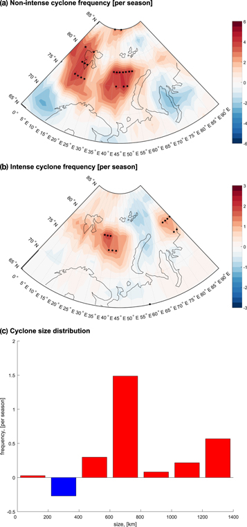
Figure 3 shows the impact of anomalous AW inflow on cyclone frequency for non-intense and intense cyclones. We find a significant increase in the frequency of occurrence for both types of cyclones over the Barents Sea. Non-intense cyclones increase over the central and western Barents Sea, while intense cyclones increase over the central Barents Sea too, where static stability decreases (figure 2(c)). Table 2 summarizes the impact of AW inflow into the Barents Sea on the frequency of cyclones. The changes are in the order of 1%–18%. The maximum influence of AW inflow on both types of cyclones is found for the months from December to March, with smaller effects in later months. However, the impact on the frequency of intense cyclone is twice as strong as on non-intense cyclones (table 2).
Figure 3. Composite difference 'High minus low AW inflow in winter' for the frequency of occurrence of (a) non-intense cyclones (depth < 20 hPa), (b) intense cyclones (depth ≥ 20 hPa) and (c) cyclone size histogram for the Barents Sea cyclones for winter (DJF). Colors show an increase (red) and a decrease (blue) of the cyclone frequency. Black dots indicate statistical significance (p < 0.05).
Download figure:
Standard image High-resolution image
Table 2. Composite difference 'high minus low AW inflow years in winter' for non-intense (cyclone depth < 20 hPa) and intense (cyclone depth ≥ 20 hPa) cyclone frequency of occurrence (%) in the Barents Sea. Statistical significant values (p < 0.05) are in bold.
| Months | DJF | JFM | FMA | MAM |
|---|---|---|---|---|
| Non-intense cyclones | 9 | 8 | 2 | 1 |
| Intense cyclones | 17 | 18 | 9 | 3 |
Figure 3(c) shows that the frequency of occurrence of cyclones increases for cyclones of almost all sizes. The strongest increase occurs for 600–800 km sized cyclones, and only small increase is seen for small-scale cyclones (radii of 100–200 km). Those small-scale cyclones are mostly associated with polar mesocyclones (Smirnova et al 2015). The only decrease appears for cyclones with radii of 200–400 km. We calculate also a significant increase in both the mean cyclone intensity (increases by ca. 5%) and cyclone size (increase by ca. 4%) over the Barents Sea. Our results for winter support the finding by Long and Perrie (2017), who noted a significant linkage between annual variation of cyclone frequency in the Barents Sea and AW inflow. However, they found only weak changes in the annual cyclone intensity.
4. Summary and conclusion
We analyzed the impact of the AW inflow on regional cyclone activity in the Barents Sea in winter using ensemble hindcast simulations from the coupled regional climate model HIRHAM-NAOSIM performed for the 1979–2016 period. The results demonstrate that increased AW inflow into the Barents Sea leads to changes in static stability and wind shear in the lower troposphere and thus favorable conditions for cyclone activity. However, the EGR does not represent a sufficient indicator of cyclone activity changes in sea ice-covered regions (e.g. Semmler et al 2016). Using the cyclone identification method, we also note an increased frequency of occurrence of cyclones, particularly of intense cyclones, in the Barents Sea in years with high AW inflow, accompanied by an increase of cyclone depth (intensity) and size. The impact of the winter (December–February) AW inflow on changes of cyclone activity is strongest from December to March.
Our results agree with earlier studies by Adakudlu and Barstad (2011) and Kolstad et al (2016, 2017) and confirm that cyclone activity (especially polar lows), in particular their intensification is sensitive to the surface conditions (SST, sea-ice) in the Barents Sea. In turn, intense cyclones significantly affect the sea ice and oceanic conditions in the Barents Sea. For example, a strong cyclone entered the Arctic at the end of December 2015, brought warm and humid air to the Barents-Kara Seas, and changed a temperature and sea ice regimes (Boisvert et al 2016). Sun and Gao (2018) also noted a key role of polar lows (from January to April) in the Barents Sea for the synoptic-scale variability of AW inflow through the Fram Strait. According to Smedsrud et al (2013) and Long and Perrie (2017), strong winds, associated with cyclones, may enhance AW inflow into the Barents Sea. However, the relative role of synoptic-scale and polar meso-scale cyclones for changing sea-ice and oceanic conditions is a complicate task due to difficulties in reproducing meso-scale cyclones by models. An interesting topic for the further analysis is to separately investigate the role of intense cyclones and polar lows for changing sea-ice and oceanic conditions in the Nordic Seas using high resolution regional climate models.
Observations as well as models indicate an increased AW inflow and associated heat transport into the Barents Sea through the BSO in recent decades (e.g. Skagseth et al 2008, Årthun et al 2012). Also, significant changes in winter cyclone activity were reported by Zahn et al (2018), with increase (decrease) in the northern (southern) Barents Sea. They also discussed an increase of cyclone depth (intensity) and size over the Barents Sea. Smirnova et al (2015) showed the positive trend in the occurrence of polar mesocyclones over the Nordic Seas. An interesting topic for the future is to investigate the potential linkages between the trends in AW inflow and the trends in cyclone activity. Due to the prescribed lateral boundary forcing, RCM simulations allow to perform targeted process studies as well as to distinguish external climate change signals from internally generated variability. This will be a topic of further studies.
Acknowledgments
The authors acknowledge the support by the project 'The linkage between polar air-sea ice-ocean interaction, Arctic climate change and Northern hemisphere weather and climate extremes (POLEX)' funded by the Russian Science Foundation (RSF No. 18-47-06203) and Helmholz association (Helmholtz-RSF). Cause-and-effect analysis was performed with the support by the Russian Science Foundation (RSF No. 19-17-00240). Support for data processing was supported by RFBR according to the research projects (No. 18-05-60216, 18-35-00091, 17-29-05098, 18-05-60111). AR and WD acknowledge the funding by the Deutsche Forschungsgemeinschaft (DFG, German Research Foundation)—Project number 268020496—TRR 172, within the Transregional Collaborative Research Center 'ArctiC Amplification: Climate Relevant Atmospheric and SurfaCe Processes, and Feedback Mechanisms (AC)3'. We also thank Professor Michael Kurgansky and Dr Alexey Eliseev for fruitful and helpful discussions.
The data that support the findings of this study are available from the corresponding author upon reasonable request.
Appendix
We use an algorithm of cyclones identification based on Bardin and Polonsky (2005) and Akperov et al (2007) with some modifications for the Arctic region (Akperov et al 2015). The algorithm is based on MSLP maps and has been applied in several other studies that investigate changes in cyclone activity in extratropical and high latitudes (Neu et al 2013, Ulbrich et al 2013, Simmonds and Rudeva 2014). Cyclones are identified as low-pressure regions enclosed by closed isobars on 6-hourly maps of MSLP. If the MSLP at one grid point is less than in the eight surrounding grid points, a candidate cyclone is identified, with its center at that grid point. To locate the outermost closed isobar, we use a pressure step of 0.1 hPa from the previous grid point to identify the locations where the pressure no longer increases. These points then make up the outermost closed isobar. With this, we are able to calculate the depth (intensity) and the size (radius) of the cyclone. The coordinates of the grid point with minimal pressure are considered as the center of the cyclones. The size (radius) is determined as the average distance from the geometric center to the outermost closed isobar. The depth (intensity) is determined as difference between the pressure in cyclone geometric center and the outermost closed isobar. For cyclone tracking, we use two thresholds–a maximum search distance (600 km) and an allowable pressure difference (20 hPa) in sequential time steps. However, we did not use any restriction on cyclone lifetime and consider all tracks (i.e. from 6 h).