
Dynamics of a Simulated Demonstration March: An Efficient Sensitivity Analysis


1
Department of Computer Science and Mathematics, Munich University of Applied Sciences, 80335 Munich, Germany
2
Department of Informatics, Technical University of Munich, 85748 Garching, Germany
*
Author to whom correspondence should be addressed.
Sustainability 2021, 13(6), 3455; https://doi.org/10.3390/su13063455
Submission received: 21 December 2020
/
Revised: 8 February 2021
/
Accepted: 17 March 2021
/
Published: 20 March 2021
(This article belongs to the Special Issue Simulations and Methods for Disaster Risk Reduction in Sustainable Built Environments)
Abstract
:Protest demonstrations are a manifestation of fundamental rights. Authorities are responsible for guiding protesters safely along predefined routes, typically set in an urban built environment. Microscopic crowd simulations support decision-makers in finding sustainable crowd management strategies. Planning routes usually requires knowledge about the length of the demonstration march. This case study quantifies the impact of two uncertain parameters, the number of protesters and the standard deviation of their free-flow speeds, on the length of a protest march through Kaiserslautern, Germany. Over 1000 participants walking through more than 100,000 m lead to a computationally demanding model that cannot be analyzed with a standard Monte Carlo ansatz. We select and apply analysis methods that are efficient for large topographies. This combination constitutes the main novelty of this paper: We compute Sobol’ indices with two different methods, based on polynomial chaos expansions, for a down-scaled version of the original set-up and compare them to Monte Carlo computations. We employ the more accurate of the approaches for the full-scale scenario. The global sensitivity analysis reveals a shift in the governing parameter from the number of protesters to the standard deviation of their free-flow speeds over time, stressing the benefits of a time-dependent analysis. We discuss typical actions, for example floats that reduce the variation of the free-flow speed, and their effectiveness in view of the findings.
1. Introduction
Protesters at demonstrations express their fundamental rights like freedom of speech [1]. As such, they are vital for democratic societies. Authorities, organizations with security tasks, and event organizers are responsible for mitigating risks and for safely guiding protesters. This necessitates the right crowd management strategies.
1.1. Microscopic Simulation of a Demonstration March
Microscopic crowd simulation is a method to model individual pedestrians. It can be seen as agent-based modeling as described in [2]. One purpose is to play through what-if scenarios, which can help evaluate and improve strategies in the planning phase. Thus, it complements expensive controlled experiments and rare systematic field observations. So far, simulations have often been used to investigate egress scenarios, while other scenarios, despite their practical relevance, are less represented. There is a particular interest in computer-based decision support for demonstration marches [3,4]. This contribution belongs in the context of the Organized Pedestrian Movement in Public Spaces (OPMoPS) project, which aims at developing a digital decision support system to improve the safety of participants at mass events as described in [5,6,7].
One key information for planning demonstration marches is the length of the demonstration march and how it evolves over time. It is necessary for the police to efficiently block side roads and to clear roads and intersections en route. Most importantly, the demonstration should not cross its own tail. If that happens, the train of marchers comes to a halt, which would necessitate last minute re-routing. To stay close to application, we investigate an event with several hundreds to over a thousand participants in a set-up inspired by real demonstrations that took place in Kaiserslautern, Germany.
Despite its great extent, the scenario must model small topographic features and pedestrians with individual characteristics to obtain realistic results for the length of the demonstration march. Only microscopic crowd simulation can capture such details.
1.2. Uncertainty Quantification in Microscopic Crowd Simulation
The results of computer simulations are subject to uncertainty. Depending on the model and its parameters, the output varies to some extent. Defining parameters for microscopic crowd models is challenging because experimental data is scarce and measurement data may be erroneous. In addition, human behavior introduces randomness into the model [8]. Such arbitrariness and lack of knowledge can affect the simulation output significantly. Neglecting variations in the output in the context of a demonstration march could lead to wrong conclusions and ultimately to decisions that may put protesters in physical danger. Therefore, input uncertainties and their effects should be quantified with suitable methods.
Typically, uncertainty is divided into aleatory uncertainty, resulting from the randomness of the observed system or model, and epistemic uncertainties, describing the modeler’s lack of knowledge [9]. We analyze epistemic uncertainties with uncertainty quantification methods. The three main approaches in the context of uncertainty quantification are solving inverse problems, forward propagation, and sensitivity analysis.
Inverse methods aim at determining the input parameter distributions such that the simulation output fits empirical data. They can be used for calibration [10,11,12]. Since there is no data available for our scenario, we focus on forward propagation and sensitivity analysis.
Forward propagation methods quantify the uncertainties in the simulation output, for example, by the moments of the probability distribution of a predefined quantity of interest. We refer the interested reader to [13] for an overview of forward propagation in fluid mechanics simulations and to [14,15,16] for a detailed theoretical foundation. As shown in [17,18,19], forward propagation methods can be used to analyze pedestrian locomotion models. von Sivers et al. [18] study a train evacuation scenario with three uncertain input parameters. They use a polynomial chaos expansion (PCE) in combination with an integration scheme to construct a surrogate model. In this manner, they save computing time when determining the uncertainty in a time-dependent model response. Dietrich et al. [17] compare Monte Carlo (MC) computations and results obtained with stochastic collocation techniques. Stochastic collocation is applied directly to the model and to a data-driven surrogate model. Again, the main goal is to speed-up computationally demanding model evaluations. Kurtc et al. [19] calculate the output uncertainty of a bottleneck scenario with a polynomial chaos expansion. They average results to account for stochastic behavior of the underlying model.
Sensitivity analysis methods provide metrics to quantify the effect of input parameters on the output. Thus, the parameters can be ranked according to importance. In particular, global sensitivity analysis is a powerful method because it allows to study the model over the whole range of the parameters, not only around a local value. In this manner, the influence of interacting parameters becomes apparent. One example for such a metric are Sobol’ sensitivity indices. Their application to bottleneck scenarios proves useful in [19,20] where small egress simulations are investigated.
In short, previous applications of forward propagation and sensitivity analysis methods to microscopic crowd simulations are few in number. Most of them use Monte Carlo techniques or polynomial chaos expansions [17,18,19,20]. Besides, uncertainty quantification methods remain limited to smaller scenarios as in [10,11,12,17,18,19,20]. To our knowledge, forward propagation and sensitivity analyses have not yet been performed on computationally demanding large scale scenarios, such as a protest demonstration, because they add to the complexity and computational effort of the problem. We wish to help close this gap, and we address the following research questions: (Q1) Which method is suited to analyze the uncertainty and sensitivity of large-scale crowd simulations? (Q2) How do the number of protesters and the protesters’ walking characteristics influence the length of a demonstration march? For this purpose, we select a suitable uncertainty quantification method for a realistic demonstration scenario by testing several approaches on a down-scaled version. We then apply the best method on the full-scale scenario. We interpret the results of the uncertainty and sensitivity analysis with respect to practical application.
1.3. Outline of the Paper
This paper is structured as follows: Section 2 introduces microscopic crowd simulation with the optimal steps model, which we use for our investigations. Besides, we briefly explain forward propagation and sensitivity analysis based on polynomial chaos expansions. In Section 3, we present the demonstration march scenario and the corresponding parameter set-up for the uncertainty quantification. We also scale down the scenario to a version for which the model can be cheaply evaluated. In Section 4, we compare uncertainty quantification results obtained with four configurations of a polynomial chaos expansion to Monte-Carlo results for the down-scaled scenario. We select the method that performs best in the benchmark to study the protest demonstration scenario in its original size. We discuss the results with respect to practical application. Section 5 summarizes the major findings and gives an outlook on future work.
2. Methods and Materials
We combine aspects of two fields of research in this contribution: crowd simulation with the optimal steps model on the one hand, forward propagation and sensitivity analysis on the other hand.
2.1. Crowd Simulation with the Optimal Steps Model
There are several approaches to simulate human crowds of which most belong to one of two categories: Macroscopic models are formulated in terms of macroscopic quantities such as flow or density. In contrast, microscopic models capture each pedestrian, or agent, individually. The latter offer a finer resolution of the crowd’s movement. We conduct our studies with an agent-based microscopic crowd simulation model, the optimal steps model [21,22] as it is implemented in the open source simulation framework Vadere [23]. Its code and design concept is publicly available on GitLab [24]. In this section, we summarize the main principles of the optimal steps model.
Like most microscopic models, the optimal steps model describes a crowd as an aggregation of virtual pedestrians, so-called agents, which move from their origins (sources) towards geographical destinations (targets). Each agent possesses individual properties to capture a real crowd’s heterogeneity. This is embodied, for example, in different walking speeds reflecting characteristics such as motivation, age, height, or fitness. In the optimal steps model, this concept is implemented with the help of the free-flow speed, which is the speed of an agent who approaches its target through a space without obstacles. The free-flow speed is also the reference for the individual stride length and stride frequency. There is a linear dependency [21]. The optimal steps model uses an event-driven update scheme: a queue within the simulation handles the stepping events for each agent.
For the agents’ navigation towards the (next) target, a navigational map is generated based on the geodesic distance between any point in the topography and the target. The map is represented by a utility function [23]. It can be interpreted as a cognitive map of the topography. Obstacles and nearby agents cause dips in utility. Each agent finds its next foot position by optimizing the utility in the area that it can reach with one step. Thus, the optimal steps model balances goals: reaching one’s target while keeping an adequate distance to other agents or obstacles.
We use the optimal steps model for locomotion because it has been carefully verified by means of unit tests. Validation against tests following the Guideline for Microscopic Evacuation Analysis [25] and comparisons to experimental data embody the second pillar of the continuous integration strategy that assures the quality of the code [23]. We believe that the qualitative results for our scenario would not alter if another state-of-the-art microscopic crowd model, be it a force based model, a velocity based model, or a rule based cellular automaton, were used.
2.2. Uncertainty Quantification Methods
In this work, we use forward propagation to study the impact of the uncertainties in the input parameters on the simulation outcome. Then, we quantify the impact of each input parameter on the simulation output by means of sensitivity analysis.
In the following sections, we refer to model f, its input x, and output y defined as
where input x represents either a single uncertain parameter or a vector of uncertain parameters. The output y is often termed quantity of interest. In this study, function f is the crowd model including the scenario set-up. The output y is a quantity computed from the simulation output, in our case, it is the length of a demonstration march.
2.2.1. Forward Propagation
Forward propagation helps to determine the likelihood of a certain output y if input x varies to some extent. For this purpose, x is treated as a random variable, and the deterministic model f is considered a stochastic model [26]. The uncertainty is propagated through the model to assess the response: with prediction intervals, the mean value and higher statistical moments, or even the full probability density function [15]. We regard our model f as a black box relying merely on model evaluations. This constitutes a non-intrusive approach. Intrusive methods would require access to the underlying code [27]. The parameter space is sampled, for example, by Monte Carlo techniques. For each sample, either model f itself, or a spectral representation of f, is evaluated. The results are collected and described statistically. Sampling based methods are advantageous because they are independent of the dimension of x. Moreover, the solution converges to the exact solution with the number of sample points . The main drawback, however, is slow convergence. For example, the Monte Carlo method converges at rate [15]. Clearly, this is only feasible if the model is computationally inexpensive.
The idea of spectral representations, such as polynomial chaos expansions [14,26], is to represent the model, which is considered a random process, by a series of orthogonal polynomials and to compute the statistics for the model output y by evaluating the expansion instead of the full model. Compared to pseudo-random Monte Carlo, polynomial chaos expansions usually need fewer model evaluations, and therefore they are computationally more efficient. However, they require a smooth relation between input and output of the model [15,26]. We assume that our model fulfills this prerequisite, since the model’s objects obey Newtonian physics. Also, from our experience with simulating crowds, we do not expect abrupt changes in the typical parameter ranges that we consider here.
2.2.2. Sensitivity Analysis
Sensitivity analysis aims to attribute the variance in the simulation output to the uncertain input parameters. Based on the parameters’ sensitivities, non-influential parameters can be fixed to reduce the complexity of the model and to save computational effort. Crucial parameters are revealed that must be chosen with high precision to reduce the uncertainty in predictive simulations [28].
We focus on global sensitivity analysis. It accounts for uncertain parameters over their full range instead of studying the effects around a fixed point as local methods do. Regression- or variance-based methods are among the most popular global techniques. We choose a variance-based approach, namely Sobol’ indices [29,30], to analyze parameter sensitivities for our model of demonstration marches. Sobol’ indices are well-established, and several convenient implementations are available [31,32]. In addition, Sobol’ sensitivity indices can be calculated from Monte Carlo samples and from spectral representations, allowing comparisons between the methods.
Sobol’ indices measure effects of each individual parameter on the simulation output as well as the effect of parameter combinations. Therefore, several indices are defined following [33,34]. First order sensitivity indices are a measure for the impact of parameter to the output variance
Similarly, sensitivity indices of second or higher order quantify the contribution of two or more interacting uncertain parameters. In practice, higher orders are often assumed to be negligible [15]. Total sensitivity indices describe the variance of the model response caused by parameter and all interactions of parameter with other parameters. This is the remaining expected variance in the output if only varies, which is equivalent to are fixed, hence
The partial variances in the numerator are normalized by the total variance , such that we obtain sensitivity indices between . A sensitivity index close to 0 indicates that the corresponding parameter has no influence, while a parameter or parameter combination with an index close to 1 dominates the output [34].
2.2.3. Polynomial Chaos Expansion Based Surrogate
The idea of polynomial chaos expansions is similar to the one behind Fourier series: A function f is approximated over a bounded interval with a series of functions. Instead of sinusoids as for Fourier series, polynomial chaos expansion uses a truncated series of polynomials . The expansion is a surrogate model for specific model outcomes, here, for the length of the demonstration march. In our case, model f depends on time t and parameter vector x, and it is approximated by
The time dependency in the coefficients is separated from the dependency on the random parameters in the polynomials. The polynomials of degree p are chosen orthogonal and according to the shape of the probability density function of the input parameters. For example, Hermite polynomials go with a normally distributed random variable x. Other types of distributions and the corresponding basis polynomials can be found in [26]. Provided that the random variables are independent in the multivariate case, it is also possible to construct orthogonal polynomials with numerical schemes as Stieltje’s recurrence relation [31].
The coefficients are computed from model evaluations, typically using the point collocation method or the pseudo-spectral approach. Point collocation employs regression methods to solve the over-determined system of equations resulting from N sample points and Equation (4). The collocation nodes are often Monte Carlo or quasi-Monte Carlo samples. The sample size is approximately , where is the minimum sample size and oversampling factor is usually chosen in [16]. Following [31,35], we define . The pseudo-spectral method approximates the coefficients by numerical integration. We use the Gaussian quadrature rule with order two times the degree of the polynomial chaos expansion to obtain sufficiently accurate polynomial coefficients. Increasing the order of the polynomial chaos only makes sense if the integration scheme is accurate enough [16]. In case of a multivariate problem, integration becomes expensive, because its cost grows exponentially with the number of random parameters. Once the polynomial coefficients are known, one can cheaply obtain statistical moments such as mean and variance from the expansion [14,15,31].
2.2.4. Python Uncertainty Quantification Tools
We use Chaospy (Version 3.3.9) [31] and SALib (Version 1.3.8) [32] for our analysis. Chaospy is an open source tool for uncertainty quantification inside the Python ecosystem. It offers well established and documented code for forward uncertainty quantification and Sobol’ decomposition of the polynomial chaos expansion. SALib allows to compute Sobol’ indices based on Sobol’ sequences instead of polynomial chaos expansions.
3. Scenario and Set-Up
In this section, we explain the structure of the study before we introduce the scenario and details about the locomotion model.
3.1. Methodology
The steps of this study are visualized in Figure 1. At first, we determine a demonstration march scenario through the city center of Kaiserslautern, Germany and derive a down-scaled version. In the following, we refer to the down-scaled scenario version as selection scenario and to the full size scenario as demonstration march scenario. Then, we address research question Q1 and identify an appropriate uncertainty quantification method (one configuration of the polynomial chaos expansion). Criteria for selecting a configuration are its accuracy in comparison to a Monte Carlo benchmark and its computational effort. Both must remain within reasonable limits. We regard a maximum relative error of for uncertainty analysis and a maximum absolute error of for the Sobol’ sensitivity indices to be accurate enough. The case study corresponds to research question Q2. We analyze the demonstration march scenario, assuming that the chosen configuration can be transferred to the same scenario in its original size and still yields correct results.
Figure 2 takes a closer look at the application of uncertainty quantification methods to our model. The black box represents the forward model, which is a simulation with the optimal steps model in Vadere. The model contains all parameters that are not considered uncertain including the topography and a fixed quantity of interest. We specify two uncertain input parameters as random variables with uniform distributions. Each evaluation of the forward model provides a measurement of the quantity of interest, the demonstration march length. A polynomial chaos expansion approximates the distribution of the time-dependent quantity of interest with a series of polynomials for each time step, and thus it replaces the forward model.
We study mainly two aspects of the simulation to learn about the parameter effects: First, the modes of the distribution of the quantity of interest are obtained using forward propagation or uncertainty analysis. Second, we derive Sobol’ indices to quantify the effect of each parameter on the output.
3.2. Demonstration March Scenario
We model part of a demonstration march that passes Richard-Wagner-Straße in Kaiserslautern, Germany. Although fictive, the scenario is realistic because protests took place in this area with similar routes [36,37,38]. First, we describe the surroundings by a simplified topography in Vadere. Figure 3 shows the modelled topography of the actual environment. We slightly adapt the topography in order to reduce the computational effort and to ensure a realistic simulation. More precisely, we add obstacles to block all side roads and thereby guarantee that all agents stay on the main route. This represents the guidance of a demonstration march along a predefined route by the police. In addition, we introduce intermediate targets, which make sure that the agents use the whole width of the street.
Second, we adapt the parameters in the simulation to fit a demonstration march. Protesters in a march often move slowly compared to leisure walking, which we account for by setting the mean free-flow speed to 0.6 m/s.
This scenario is computationally demanding due to the large dimensions of the topography and the number of simulated agents. Therefore, we define a small version in order to run preliminary studies at low cost and transfer the insights to the original size scenario.
3.3. Selection Scenario: A Down-Scaled Demonstration March
The selection scenario is a down-scaled version of the demonstration march through Richard-Wagner-Straße as described before. In order to maintain similar dynamics, we have to avoid too narrow corridors. Therefore, we choose a minimal street width of 5 m and scale the area of the topography accordingly by a factor . Analogously, the number of agents is reduced by C as well. Table 1 shows the set-up for the selection and the demonstration scenario. Evaluating the selection scenario is about 50 times faster than the demonstration scenario. This allows numerous evaluations of the model, for example to generate reference solutions.
3.4. Uncertain Input Parameters
We expect the number of agents and the standard deviation of their free-flow speed to have significant influence on the quantity of interest, which means that uncertainties in these quantities could lead to great variations in the output. Previous work [39] supports this assumption. Generally, these two parameters are important in the field of pedestrian dynamics as indicated by the multitude of related contributions. Just to name a few, Bode [10], Kurtc et al. [19], Dietrich et al. [17], Corbetta et al. [12], and Fujita et al. [40] address the pedestrians’ speed or number, albeit in a different context or with different methods. It would be interesting to take more parameters into account. However, increasing the parameter space quickly evokes the curse of dimensionality. We keep the computational effort low in our first study to focus on the actual aim. Therefore, we consider these two parameters uncertain. This implicates that they are treated as random variables. Assuming a uniform distribution is a typical approach when one does not have any information on the true distributions. Table 2 lists the parameter ranges that define the input uncertainty. All other parameters are fixed. The configuration is described in Appendix A.
The standard deviation of free-flow speed is a central parameter in pedestrian locomotion models as it represents a measure for the variation of the speeds among the pedestrians when they approach their targets without hindrance. A homogeneous group is characterized by a low standard deviation. In contrast, a heterogeneous crowd with participants, for example, of different fitness, motivation, or age can be described by a greater standard deviation of the free-flow speed. We assume that participants of a protest demonstration move at a similar speed. That is, we expect the standard deviation of the pedestrians’ speed distribution to be significantly lower than 0.26 m/s, a typical value for normal traffic situations [41] and the default in Vadere [23]. Bearing in mind that the parameter range must be sufficiently large for a meaningful sensitivity analysis, we set m/s as lower bound and m/s as upper bound.
The number of agents, or demonstrators, is regarded as an uncertain parameter because it is often unknown how many protesters actually attend a demonstration. In fact, expectations and reality may diverge drastically, which constitutes a major problem for the police and other entities. The number of participants depends on several factors, for example, recurrence of the event, competing events, weather, and weather forecast. We model a typical demonstration in the area of our scenario, such as Fridays For Future demonstrations with several hundred to thousand protesters as described in [37,38]. Therefore, we define an interval from 400 to 1200 agents.
3.5. Definition and Computation of the Quantity of Interest: Length of the Demonstration March
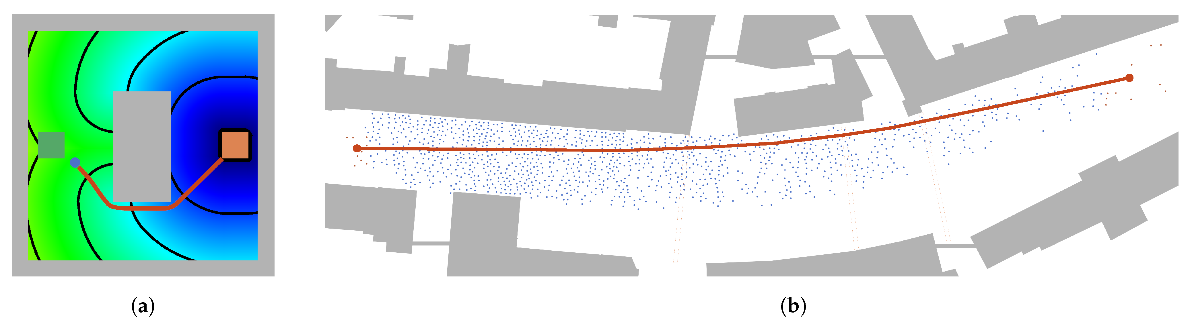
Our study focuses on the length of a demonstration march. We define the length of the demonstration march as the distance between the front and the rear of the march. It is measured by means of the geodesic distance, as in previous work [39]. In contrast to the Euclidean distance, the geodesic distance takes the topography, in particular obstacles, into account.
Each agent has a certain potential according to the current position on the floorfield. The potential represents the geodesic distance between the agent and its target at all times t. Hence, the length of the demonstration march can be approximated by
provided that and relate to agents at the front and at the rear of the march, respectively.
Due to the different free-flow speeds, some agents outrun the others or fall behind. For a more robust determination of front and rear of the march, we use the average geodesic distance of the first and last k agents. The length of the demonstration march is then defined by
with . We choose as a compromise between a sufficiently accurate estimate for the length and a reasonable number of agents that can be regarded as front and rear of the march. The measure is visualized in Figure 4b.
3.6. Handling the Stochastic Initialization
While the core of the optimal steps model is deterministic, the initialization is typically stochastic. The starting positions as well as free-flow speeds are assigned randomly due to lack of knowledge. This stochastic initialization is one way to handle the aleatory uncertainty, similar to the behavioral uncertainty defined in [8]. Polynomial chaos expansions as well as calculation of Sobol’ indices, however, require deterministic model evaluations. Therefore, we follow the approach in [19] and average repeated model evaluations at each sample point. Ideally, the number of runs would be chosen based on convergence criteria as presented in [8]. Since our scenario is computationally expensive, we take a pragmatic approach and average 10 repetitions in order to keep the analysis feasible.
4. Computational Results and Discussion
Now, we use the selection scenario to identify an appropriate configuration of the polynomial chaos expansion for the subsequent case study of the demonstration scenario. We apply different configurations of polynomial chaos expansions to the selection scenario, conduct the analysis for them, and compare the results to a benchmark with a classical pseudo-random Monte Carlo approach. Then, we select the most accurate configuration for the actual case study. This is necessary because running the demonstration march scenario demands too much computing capacity to be examined with Monte Carlo techniques. In contrast, the surrogate model constructed with polynomial chaos expansions can be evaluated cheaply. The construction is performed for each time step because the quantity of interest is time-dependent. Finally, we discuss the computational results and their implications for typical actions taken in practice to complement the case study.
4.1. Selecting a Configuration for the Polynomial Chaos Expansion
There are two common approaches to determine the coefficients of the polynomial chaos expansion, the point collocation method and the pseudo-spectral projection. Important characteristic numbers of the expansions are the polynomial degree p, the oversampling factor for point collocation, and the order of the quadrature rule for the pseudo-spectral approach. These three factors determine the sample size, and thus the computational effort. High polynomial orders lead to large samples but do not necessarily improve the accuracy of the expansion. We use randomly sampled nodes for the point collocation method, and therefore we can choose the sample size arbitrarily, while the sample points for the pseudo-spectral approach are determined by the order of the quadrature rule. In this case, we obtain larger samples for the pseudo-spectral method.
For both methods, we compare the approximation with polynomial degrees 2 and 3, as described in Table 3. More precisely, we compare the results for each configuration to a reference solution. First, we look at the mean and standard deviation over all samples of the length of the demonstration march. The reference solution for these is generated with classical pseudo-random Monte Carlo samples. Then, we compute sensitivity indices. We obtain the reference indices with Saltelli’s extension of the Sobol’ sequence [32,34] with a total number of sample points. These sample sizes lead to sufficiently converged results (see Appendix B). Looking at both the error in the forward propagation results and the errors in the sensitivity indices as quantitative measures, the pseudo-spectral approach with 3rd order polynomials and sample size of (configuration PS-3) yields the most accurate results.
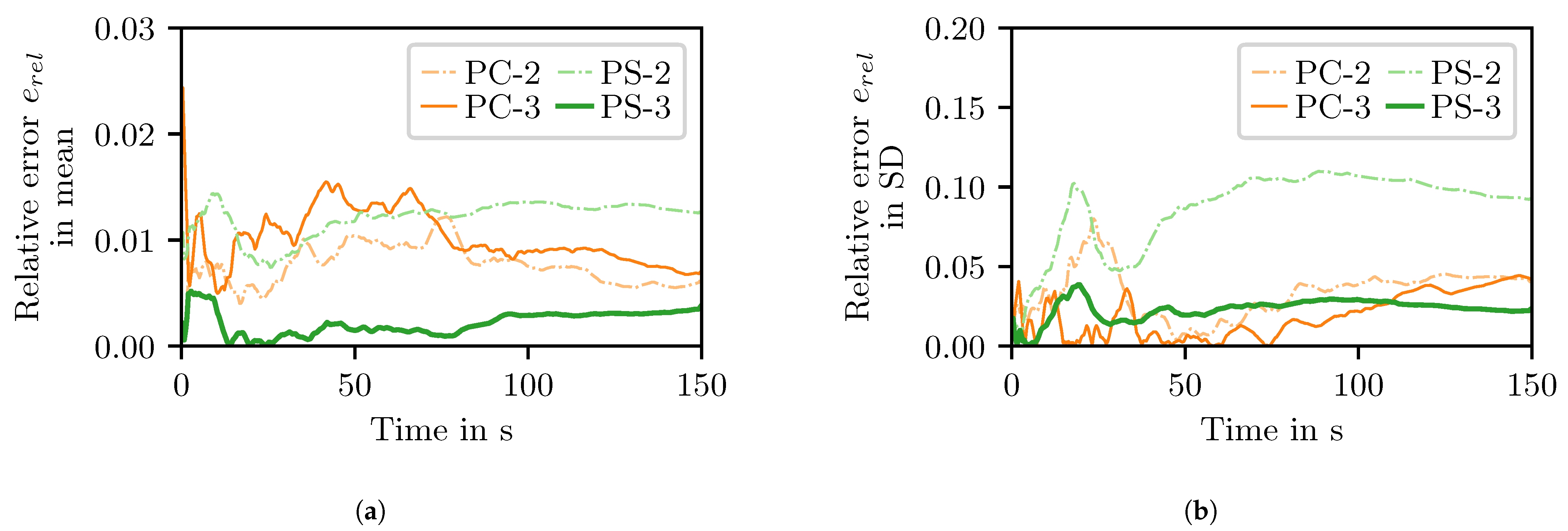
For each configuration, we compute the relative error in the mean over all samples and the standard deviation over all samples for the length of the demonstration march: . In the formula, y stands for the mean or the standard deviation and indicates the reference solution. Figure 5 shows that the relative error in the mean is less than , which is negligible. The relative error in the standard deviation for the configuration PS-3 of the surrogate is less than , and therefore still acceptable.
The sensitivity indices range in . Thus, it makes sense to look at the absolute error . Figure 6 reveals that configuration PS-3 tends to under- or overestimate the sensitivity indices, but the deviation remains within reasonable limits.
Our quantitative and qualitative comparisons (see Appendix C for more details) show that the polynomial chaos expansion yields sufficiently accurate results in the selection scenario, and thus it can replace expensive Monte Carlo computations. Consequently, we select the pseudo-spectral configuration with polynomial order and sample points (PS-3), which performed best in the benchmark, for the full-scale analysis. We argue that both scenarios exhibit similar dynamics, and therefore the method can be transferred.
A solution obtained with classical Monte Carlo requires more than 400 up to 2000 sample points to reach a similar accuracy as the polynomial chaos expansion with (see Appendix B). Thus, we save eight to 41 times the computational effort that is necessary for evaluating to 2000 Monte Carlo samples, respectively. This comparison does not take into account constructing the surrogate with polynomial chaos expansions because the model evaluations dominate the total computing time.
4.2. Case Study: A Realistic Demonstration March through a City Center
In this section, we perform forward propagation and analyze the sensitivity the of length of the demonstration march for the full-scale scenario. We apply polynomial chaos expansion with 3rd order polynomials in combination with the pseudo-spectral approach. The nodes are sampled according to a 7 point Gaussian quadrature rule, which leads to sample points. From the polynomial expansion, that is, from our surrogate model we calculate mean and standard deviation as well as the Sobol’ sensitivity indices. Finally, we interpret the forward propagation and the sensitivity analysis results with respect to practical application.
4.2.1. Forward Propagation
We use mean and standard deviation to quantify the uncertainty in the length of the demonstration march. The demonstration march scenario exhibits the same dynamics in the output uncertainty as the selection scenario (compare Figure 7 and Figure A4).
The length of the demonstration march increases over time and the standard deviation increases during most of the time. Appearance of agents in the source and disappearance in the destination can cause artifacts in the beginning and end of the simulations. Therefore, we restrict our observations to the time interval (measured in seconds) in which the agents have already started forming a demonstration march but have not yet reached their target.
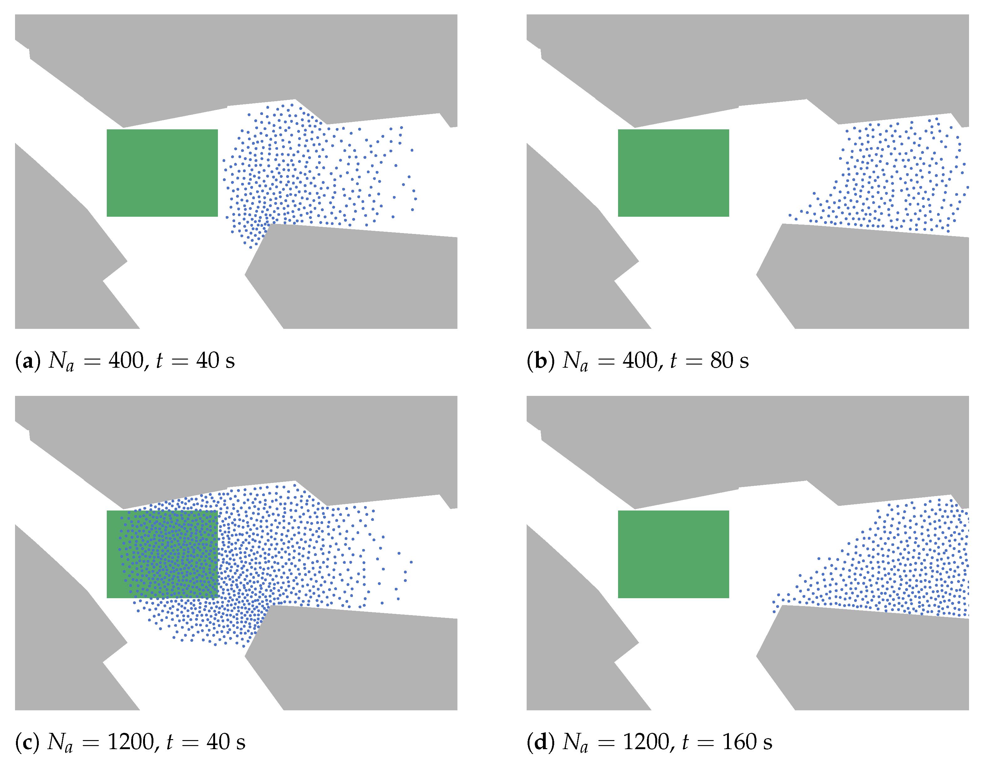
The evolution of the standard deviation of the length of the march and especially its minimum around 50 s may be surprising at first. Both are a result of the forming process of the demonstration march visualized in Figure 8. In the beginning, all agents are in or closely around the source, similar to the participants of a demonstration gathering in a public place. Thus, until all agents have left the source (≥160 s, compare Figure 8d), the results must be interpreted carefully. Once the demonstration march has formed, we observe an almost linear increase of the demonstration march length. All results indicate that a time-dependent analysis is necessary to grasp the characteristics of the system.
In reality, roughly estimated quantities, such as the number of protesters and their heterogeneous walking habits, lead to output uncertainties expressed by demonstration marches of different length. This does not allow for reliable statements. However, forward propagation enables us to derive a probable length, for example (t = 450 s) = 150 m, and to be aware of realistic deviations. In this case the standard deviation represents about of the mean.
4.2.2. Global Sensitivity Analysis
The sensitivity indices express the influence of the two parameters, standard deviation of the free-flow speed and number of agents, on the length of the demonstration march. Figure 9 plots the total order sensitivity index . The difference between the first order index and the total order index is negligible (compare Figure 9 and Figure A6). That means, first order contributions dominate the total sensitivity and interaction effects between the two uncertain parameters barely add to the uncertainty in the output. Therefore, we focus only on the total sensitivities.
In the beginning, the standard deviation of free-flow speed has no impact on the length of the demonstration march, while the number of agents is the all-dominant factor. This relation shifts over time so that at the end of the simulation the standard deviation of free-flow speed is dominant. Usually, routes for demonstration marches are longer than a few hundred meters, but we consider only a part of a realistic demonstration. We assume that, in case of a longer demonstration route, the influence of parameter 1 and 2 would follow the trend in Figure 9 and approach 1 and 0, respectively.
The small peak at around s coincides with the local minimum of the standard deviation of the quantity of interest (Figure 7) and can be traced back to the topography. When the first agents start moving while the rear of the march stands still, the standard deviation quickly gains influence. However, there is a corner that the agents in the lower part of Figure 8 must pass, causing a small congestion that hinders faster agents. Once all agents move and have cleared the obstacle, the influence of the standard deviation of the speed grows monotonously.
Our findings implicate that the number of participants determines the extent of the demonstration march in the beginning, but the influence declines as soon as the protesters start moving. The difference in the protesters’ walking speeds come more and more into effect the longer the route is. The next step is to transfer this information to the measures that the police builds upon to guide and protect the crowd.
4.2.3. Discussion: Relevance with Respect to Practical Application
So far, we have analyzed our results with respect to the simulation. Now, we focus on the implications of the uncertainty and sensitivity analysis for practical application. We discuss the results in view of common measures to control the length of a demonstration march.
We observed that the topography has an impact on the length of the demonstration march. In particular, even a seemingly minor bottleneck, such as the narrowing of a street, compresses the demonstration march locally. This leads to higher densities, which may endanger the pedestrians and should be avoided. It also elongates the march when the head of the march moves away from the main crowd at the holdup. The different flow conditions in the northern part of the demonstration scenarios, which resembles a bottleneck, and the straight southern part of the scenario support the use of physical barriers to smooth the boundaries, and thus to prevent congestion.
At the beginning of the march, the number of agents is the dominant parameter, but its importance decreases over time. In practice, this parameter cannot be regulated easily. One measure is limiting the number of participants by the organizer or local authorities. However, even with that, the actual number of protesters often deviates from the announcement or permit. Hence, we suggest to run through what-if scenarios for a range of participant numbers in the planning phase and to devise contingency plans for worst case scenarios.
We find that the standard deviation of the agents’ free-flow speed dominates the length of the demonstration march in the long run. Measures that reduce the variation of the free-flow speed among the protesters keep the demonstration compact. Floats and banners at different positions within the march are common measures to synchronize the participants’ speeds. So are front runners and helpers at the back who urge dawdlers on. Our findings confirm how useful these measures are and justify their costs.
5. Conclusions and Outlook
We simulated a demonstration march through the city center of Kaiserslautern, Germany, using a state-of-the art pedestrian dynamics model. We quantified the impact of two important but uncertain parameters on the length of the demonstration march: the number of participants, or agents, and the standard deviation of their free-flow speeds. The length of the march is a quantity of great practical interest.
The demonstration march is a large-scale and computationally expensive scenario. Analyzing it statistically meant drawing many samples. With the help of a down-scaled version of the model we selected a configuration for an efficient surrogate model, a polynomial chaos expansion, of the quantity of interest. For this purpose, we compared the performance of several surrogate configurations to a benchmark where we used classical pseudo-random Monte Carlo sampling. Then we employed the most accurate configuration to compute a polynomial chaos expansion of the model in its original size. We needed eight to 41 times fewer model evaluations for the construction of the surrogate than classical Monte Carlo sampling would have required. Thus, we were able to conduct a full analysis.
Forward propagation of uncertain parameters showed that the output uncertainty, characterized by the mean and the standard deviation of the length of the march, increased over simulation time. The sensitivity analysis with Sobol’ indices revealed that, in the beginning, the number of agents dominated the march length, whereas the standard deviation of free-flow speed prevailed in the long run. This proves that time-dependent analysis is necessary to grasp the characteristics of the system.
Our results scientifically confirmed the usefulness of measures to reduce the variation in the walking speeds of the participants. It also justified the expense for deploying orderlies at demonstrations. Besides, it emphasized that it is essential to run through a number of what-if scenarios with very different numbers of participants so that routes of suitable lengths can be assigned, and contingency plans can be devised. Our findings demonstrate how uncertainty quantification through simulations can become a corner stone of a computer-based decision support system for the planning of large events.
We are aware of several limitations of our study: It would be helpful to simulate even bigger scenarios and over longer time periods. Moreover, we treated the crowd as an aggregation of individuals while, in reality, protesters form groups. We aim to overcome these limitations in future work. We also plan to consider additional parameters that we believe influential. Among these the participants’ need for personal space, that is, the distance one tries to maintain to unknown other agents, has gained urgent attention in the context of the spread of infectious diseases during public events.
Author Contributions
Conceptualization, G.K., M.G., R.F., and S.R.; methodology, M.G., R.F., and S.R.; software, S.R.; validation, S.R.; formal analysis, M.G. and S.R.; investigation, S.R.; resources, G.K.; data curation, S.R.; writing—original draft preparation, M.G. and S.R.; writing—review and editing, G.K., M.G., R.F., and S.R.; visualization, S.R.; supervision, G.K, M.G., and R.F.; project administration, G.K.; funding acquisition, G.K. All authors have read and agreed to the published version of the manuscript.
Funding
This research was funded by the German Federal Ministry of Education and Research grant number 13N14562. The APC was funded by the Open Access Publication fund of the Munich University of Applied Sciences.
Acknowledgments
The authors would like to thank Benedikt Kleinmeier for discussions on modelling the demonstration scenario and Daniel Lehmberg for providing the SUQcontroller as a part of the Vadere framework. The authors acknowledge the support by the research office FORWIN at the Munich University of Applied Sciences.
Conflicts of Interest
The authors declare no conflict of interest.
Appendix A. Scenario Set-Up
As described in Section 3, we consider two parameters uncertain. Other parameters are set to their default values as defined in Vadere [24] except the ones listed in Table A1. These parameters define a normal distribution of the agents’ free-flow speed truncated at minimumSpeed and maximumSpeed to avoid implausible values. We expect that participants of a demonstration have lower minimum, mean, and maximum free-flow speeds, so we adapt the parameters accordingly.

Table A1.
Modified speed distribution parameters in the Vadere code (measured in m/s).
| Variable | Default Value | Defined Value |
|---|---|---|
| speedDistributionMean | ||
| speedDistributionStandardDeviation | ||
| minimumSpeed | ||
| maximumSpeed |
Besides, we use the cache function (cacheType: BIN_CACHE) in Vadere, and thus we speed-up the model evaluation of both scenarios. The scenario files are available in Vadere [24].
To ensure that the model output can be reproduced by third parties, we define fixed seeds for each repeated model evaluation for the same sample as described in Section 3.6. The seeds listed in Table A2 are chosen randomly.
Table A2.
Simulation seeds used for repeated model evaluations of the same sample.
| Run | Simulation Seed |
|---|---|
| 1 | −4800259349912033156 |
| 2 | 4102095800580213524 |
| 3 | −1188124012262499647 |
| 4 | 5776439357318270195 |
| 5 | 227024315392238807 |
| 6 | −6081968063774661054 |
| 7 | −3437215030857689178 |
| 8 | 5619284164153179787 |
| 9 | 3989138166911000642 |
| 10 | −1646650504514963182 |
Appendix B. Calculation of a Reference Solution for the Selection Scenario
In Section 4.1, we compare four configurations of the polynomial chaos expansion to a reference solution, treated as ground truth. Figure A1 shows the convergence of the mean over all samples and standard deviation over all samples of the output, that is, the length of the demonstration march. We consider the forward propagation results for to be converged because they deviate less than from the results for . We use the results for mean and standard deviation obtained with as reference solution.
Figure A1.
Forward propagation results for the down-scaled scenario obtained with pseudo-random Monte Carlo samples. (a) Mean over all samples of the length of the demonstration march; (b) Standard deviation over all samples of the length of the demonstration march.
Figure A1.
Forward propagation results for the down-scaled scenario obtained with pseudo-random Monte Carlo samples. (a) Mean over all samples of the length of the demonstration march; (b) Standard deviation over all samples of the length of the demonstration march.

Figure A2 shows the convergence of the sensitivity indices. Using SALib allows to employ Sobol’ sequences. In our case, the Sobol’ sequence yields more accurate results than a sampling scheme based on the same samples used for the forward propagation. The sensitivity indices for are regarded as converged because they deviate less than from the results for . We use the sensitivity indices obtained with as reference solution.
Figure A2.
Sensitivity indices for the down-scaled scenario obtained with Sobol’ sequences and a total number of N sample points. (a) First order sensitivity index for the standard deviation of free-flow speed; (b) First order sensitivity index for the number of agents; (c) Total sensitivity index for the standard deviation of free-flow speed; (d) Total sensitivity index for the number of agents.

We compare the computational effort of uncertainty quantification with Monte Carlo and polynomial chaos expansions. For this purpose, we identify a configuration of Monte Carlo that reaches the required accuracy of maximum absolute error as defined in Section 3.1: The indices for deviate up to from the reference solution in the worst case. That means, sample points are almost sufficient, but only the configuration with indeed meet the requirements.
Appendix C. Comparison of the Reference Solution and the Polynomial Chaos Expansion Applied to the Selection Scenario
The distribution of the model output is approximated for each time step with four configurations of the polynomial chaos expansion. Figure A3 shows the distributions for equally distanced time steps within the time interval (measured in seconds). The qualitative comparison reveals that the polynomial chaos expansions with PC-2, PS-2, and PS-3 fit the reference solution well.
Figure A3.
The uncertainty in the model output is represented by distributions for selected time steps t. The configurations of the polynomial chaos expansions are PC-2 (PC, , ), PC-3 (PC, , ), PS-2 (PS, , ), and PS-3 (PS, , ). The histogram represents the reference solution (MC), which is generated with pseudo-random Monte Carlo samples ().

It is more comfortable to compare statistical moments calculated from the distributions than the full probability density function for each time step because statistical moments can be captured by a single graph. Figure A4 shows the approximation of mean and standard deviation of the demonstration march length with the four configurations for the polynomial chaos expansion. As expected, the length of the demonstration march increases over time due to the different walking speeds.
Figure A4.
Mean (a) and standard deviation (b) of the length of the demonstration march obtained with configurations of the polynomial chaos expansion PC-2 (PC, , ), PC-3 (PC, , ), PS-2 (PS, , ), and PS-3 (PS, , ). The reference solution (MC) is generated with pseudo-random Monte Carlo samples ().
Figure A4.
Mean (a) and standard deviation (b) of the length of the demonstration march obtained with configurations of the polynomial chaos expansion PC-2 (PC, , ), PC-3 (PC, , ), PS-2 (PS, , ), and PS-3 (PS, , ). The reference solution (MC) is generated with pseudo-random Monte Carlo samples ().

Figure A5 shows the sensitivity indices for selection scenario. The indices for the standard deviation of the free-flow speed and the number of agents reveal that the demonstration march length is driven by the number of agents in the beginning of the demonstration, but over time, the variation in free-flow speeds increases in importance while the effect of the number of agents decreases.
Figure A5.
Sensitivity indices for the standard deviation of free-flow speed and number of agents obtained with configurations of the polynomial chaos expansion PC-2 (PC, , ), PC-3 (PC, , ), PS-2 (PS, , ), and PS-3 (PS, , ) for sensitivity indices of the standard deviation of free-flow speed and the number of agents. The reference solution (MC) is generated with a Sobol’ sequence with a total number of sample points. (a) First order sensitivity index for the standard deviation of free-flow speed; (b) First order sensitivity index for the number of agents; (c) Total sensitivity index for the standard deviation of free-flow speed; (d) Total sensitivity index for the number of agents.

Appendix D. First Order Sensitivity Indices for the Demonstration Scenario
The sensitivity analysis of the demonstration scenario in Section 4.2.2 yields similar results for both total sensitivity indices and first order sensitivity indices (compare Figure 9 and Figure A6). First order sensitivity indices quantify only the influence of a single parameter on the output.
Figure A6.
First order sensitivity indices quantifying the importance of each input parameter.

References
- Charter of Fundamental Rights of the European Union. Off. J. Eur. Union 2012, C326, 391–407.
- Bonabeau, E. Agent-based modeling: Methods and techniques for simulating human systems. Proc. Natl. Acad. Sci. USA 2002, 99, 7280–7287. [Google Scholar] [CrossRef] [PubMed] [Green Version]
- Hauff, L. Polizeiliches Handeln und Denken im Einsatz. Warum wissenschaftliche Zusammenarbeit mit der Polizei eine Herausforderung ist und warum es sich trotzdem lohnt—Das Beispiel Rheinland-Pfalz. 2021. Available online: https://crisis-prevention.de/innere-sicherheit/polizeiliches-handeln-denken-im-einsatz.html (accessed on 19 March 2021).
- Kubera, T. Was bringen IT-gestützte Simulationsverfahren der Polizei? Ein Situationsbericht aus Sicht der Deutschen Hochschule der Polizei. Polizei, Verkehr + Technik 2014, 1, 7–11. [Google Scholar]
- Munich University of Applied Sciences. Munich University of Applied Sciences—Research Project—OPMOPS—Organized Pedestrian Movement in Public Spaces. 2020. Available online: https://www.hm.edu/en/research/projects/project_details/koester_1/details_opmops.en.html (accessed on 19 March 2021).
- Bundesministerium für Bildung und Forschung. OPMOPS: Organisierte Umzüge und Demonstrationen im Öffentlichen Raum: Planung und Krisenmanagement bei hohem Konfliktpotenzial in Städten—BMBF Sicherheitsforschung. 2020. Available online: https://www.sifo.de/de/opmops-organisierte-umzuege-und-demonstrationen-im-oeffentlichen-raum-planung-und-2451.html (accessed on 19 March 2021).
- Hamacher, H.; Ruzika, S. OPMoPS—TU Kaiserslautern. 2020. Available online: https://www.mathematik.uni-kl.de/en/opt/research/research-projects/opmops/ (accessed on 19 March 2020).
- Ronchi, E.; Kuligowski, E.D.; Reneke, P.A.; Peacock, R.D.; Nilsson, D. The Process of Verification and Validation of Building Fire Evacuation Models; Technical Note 1822; National Institute of Standards and Technology (NIST), U. S. Department of Commerce: Gaithersburg, MD, USA, 2013. [CrossRef] [Green Version]
- Oberkampf, W.L.; Roy, C.J. Verification and Validation in Scientific Computing; Cambridge University Press: Cambridge, UK, 2010. [Google Scholar]
- Bode, N. Parameter Calibration in Crowd Simulation Models using Approximate Bayesian Computation. Collect. Dyn. 2020, 5. [Google Scholar] [CrossRef]
- Gödel, M.; Fischer, R.; Köster, G. Applying Bayesian inversion with Markov Chain Monte Carlo to Pedestrian Dynamics. In Proceedings of the UNCECOMP 2019, 3rd ECCOMAS Thematic Conference on Uncertainty Quantification in Computational Sciences and Engineering, Crete, Greece, 24–26 June 2019. [Google Scholar] [CrossRef]
- Corbetta, A.; Muntean, A.; Vafayi, K. Parameter Estimation of Social Forces in Pedestrian Dynamics Models via a Probabilistic Method. Math. Biosci. Eng. 2015, 12. [Google Scholar] [CrossRef] [PubMed]
- Iaccarino, G. Quantification of Uncertainty in Flow Simulations Using Probabilistic Methods; VKI Lecture Series; Mechanical Engineering Institute for Computational Mathematical Engineering Stanford University: Stanford, CA, USA, 2008. [Google Scholar]
- Xiu, D. Numerical Methods for Stochastic Computations: A Spectral Method Approach; Princeton University Press: Princeton, NJ, USA, 2010. [Google Scholar]
- Smith, R.C. Uncertainty Quantification: Theory, Implementation, and Applications; Computational Science and Engineering; Society for Industrial and Applied Mathematics: Philadelphia, PA, USA, 2014. [Google Scholar]
- Xiu, D. Stochastic Collocation Methods: A Survey. In Handbook of Uncertainty Quantification; Ghanem, R., Owhadi, H., Higdon, D., Eds.; Springer International Publishing: Cham, Switzerland, 2017; Volume 45, pp. 699–716. [Google Scholar] [CrossRef]
- Dietrich, F.; Künzner, F.; Neckel, T.; Köster, G.; Bungartz, H.J. Fast and flexible uncertainty quantification through a data-driven surrogate model. Int. J. Uncert. Quantif. 2018, 8, 175–192. [Google Scholar] [CrossRef]
- von Sivers, I.K.M.; Templeton, A.; Künzner, F.; Köster, G.; Drury, J.; Philippides, A.; Neckel, T.; Bungartz, H.J. Modelling social identification and helping in evacuation simulation. Saf. Sci. 2016, 89, 288–300. [Google Scholar] [CrossRef] [Green Version]
- Kurtc, V.; Köster, G.; Fischer, R. Sensitivity Analysis for Resilient Safety Design: Application to a Bottleneck Scenario; Springer: Singapore, 2020; pp. 255–264. [Google Scholar] [CrossRef]
- Gödel, M.; Fischer, R.; Köster, G. Sensitivity Analysis for Microscopic Crowd Simulation. Algorithms 2020, 13, 162. [Google Scholar] [CrossRef]
- Seitz, M.J.; Köster, G. Natural discretization of pedestrian movement in continuous space. Phys. Rev. E 2012, 86, 046108. [Google Scholar] [CrossRef] [PubMed]
- von Sivers, I.; Köster, G. Dynamic Stride Length Adaptation According to Utility And Personal Space. Transp. Res. Part B Methodol. 2015, 74, 104–117. [Google Scholar] [CrossRef] [Green Version]
- Kleinmeier, B.; Zönnchen, B.; Gödel, M.; Köster, G. Vadere: An Open-Source Simulation Framework to Promote Interdisciplinary Understanding. Collect. Dyn. 2019, 4. [Google Scholar] [CrossRef] [Green Version]
- Vadere. 2020. Commit Hash: 72924185. Available online: https://gitlab.lrz.de/vadere/vadere/tags/Paper_dynamics_demonstration_march (accessed on 19 March 2021).
- RiMEA. Guideline for Microscopic Evacuation Analysis, RiMEA e.V., 3.0.0 ed. 2016. Available online: https://rimeaweb.files.wordpress.com/2016/06/rimea_richtlinie_3-0-0_-_d-e.pdf (accessed on 19 March 2021).
- Xiu, D. Fast numerical methods for stochastic computations: A review. Commun. Comput. Phys. 2009, 5, 242–272. [Google Scholar]
- Sudret, B. Global sensitivity analysis using polynomial chaos expansions. Reliab. Eng. Syst. Saf. 2008, 93, 964–979. [Google Scholar] [CrossRef]
- Saltelli, A.; Ratto, M.; Andres, T.; Campolongo, F.; Cariboni, J.; Gatelli, D.; Saisana, M.; Tarantola, S. Global Sensitivity Analysis. The Primer; John Wiley & Sons, Ltd.: Hoboken, NJ, USA, 2008; pp. 1–292. [Google Scholar] [CrossRef] [Green Version]
- Sobol’, I. Sensitivity estimates for nonlinear mathematical models. Math. Model. Comput. Exp. 1993, 1, 407–414. [Google Scholar]
- Homma, T.; Saltelli, A. Importance measures in global sensitivity analysis of nonlinear models. Reliab. Eng. Syst. Saf. 1996, 52, 1–17. [Google Scholar] [CrossRef]
- Feinberg, J.; Langtangen, H.P. Chaospy: An open source tool for designing methods of uncertainty quantification. J. Comput. Sci. 2015, 11, 46–57. [Google Scholar] [CrossRef] [Green Version]
- Herman, J.; Usher, W. SALib: An open-source Python library for Sensitivity Analysis. J. Open Source Softw. 2017, 2. [Google Scholar] [CrossRef]
- Saltelli, A. Making best use of model evaluations to compute sensitivity indices. Comput. Phys. Commun. 2002, 145, 280–297. [Google Scholar] [CrossRef]
- Saltelli, A.; Annoni, P.; Azzini, I.; Campolongo, F.; Ratto, M.; Tarantola, S. Variance based sensitivity analysis of model output. Design and estimator for the total sensitivity index. Comput. Phys. Commun. 2010, 181, 259–270. [Google Scholar] [CrossRef]
- Hosder, S.; Walters, R.W.; Balch, M. Efficient Sampling for Non-Intrusive Polynomial Chaos Applications with Multiple Uncertain Input Variables. In Proceedings of the 48th AIAA/ASME/ASCE/AHS/ASC Structures, Structural Dynamics, and Materials Conference, Honolulu, HI, USA, 23–26 April 2007. [Google Scholar] [CrossRef]
- Ditt, R. Kaiserslautern Kompakt: Demo in der Innenstadt. 2015. Available online: https://www.rheinpfalz.de/lokal/kaiserslautern_artikel,-kaiserslautern-kompakt-demo-in-der-innenstadt-_arid,367551.html (accessed on 19 March 2021).
- Ginkel, B. Demonstranten fordern mehr Grün und mehr Platz für Radfahrer in Kaiserslautern. 2020. Available online: https://www.rheinpfalz.de/lokal/kaiserslautern_artikel,-demonstranten-fordern-mehr-gr%C3%BCn-und-mehr-platz-f%C3%BCr-radfahrer-in-kaiserslautern-_arid,5115008.html (accessed on 19 March 2021).
- Vollmer, J. Fridays for Future Demonstration in Kaiserslautern. 2019. Available online: https://www.wochenblatt-reporter.de/kaiserslautern/c-lokales/fridays-for-future-demonstration-in-kaiserslautern_a125044 (accessed on 19 March 2021).
- Rahn, S. Uncertainty Quantification in Microscopic Crowd Simulation Based on Polynomial Chaos Expansion. Master’s Thesis, Munich University of Applied Sciences, Munich, Germany, 2020. Available online: https://nbn-resolving.org/urn:nbn:de:bvb:m347-dtl-0000001907 (accessed on 19 March 2021).
- Fujita, A.; Feliciani, C.; Yanagisawa, D.; Nishinari, K. Traffic flow in a crowd of pedestrians walking at different speeds. Phys. Rev. E 2019, 99, 062307. [Google Scholar] [CrossRef] [PubMed]
- Weidmann, U. Transporttechnik der Fussgänger, 2nd ed.; Volume 90 Schriftenreihe des IVT; Institut für Verkehrsplanung, Transporttechnik, Strassen- und Eisenbahnbau (IVT) ETH: Zürich, Germany, 1992. [Google Scholar] [CrossRef]
Figure 1.
The partitioned structure of this study reflects research question Q1 (blue) and research question Q2 (orange). The methods applied are polynomial chaos expansions (PCE) and classical Monte Carlo (MC) computations.
Figure 1.
The partitioned structure of this study reflects research question Q1 (blue) and research question Q2 (orange). The methods applied are polynomial chaos expansions (PCE) and classical Monte Carlo (MC) computations.

Figure 2.
Flow chart visualizing forward propagation and sensitivity analysis with polynomial chaos expansions: The uncertainty of two input parameters, number of agents and standard deviation (SD) of the agents’ free-flow speeds, is propagated through the model regarded as black box. The resulting output uncertainty is approximated by polynomial chaos expansions for each time step, which allow to calculate measures of uncertainty and sensitivity.

Figure 3.
The map shows the northern part of Richard-Wagner-Straße, Kaiserslautern, (rotated ccw.). The topography is a simplified version of the actual environment. Agents start from the source (green rectangle), pass four intermediate targets (orange lines) before they reach their final target (orange polygon).

Figure 4.
The approximate length of the demonstration march (b) is measured by means of the geodesic distance (a), which represents the shortest path around obstacles (grey), between agents (blue), and target (orange).
Figure 4.
The approximate length of the demonstration march (b) is measured by means of the geodesic distance (a), which represents the shortest path around obstacles (grey), between agents (blue), and target (orange).

Figure 5.
Relative errors in forward propagation when benchmark results from a Monte Carlo approach are compared to results obtained with polynomial chaos expansions as surrogates. The relative errors are computed for the mean over all samples (a) and standard deviation over all samples (b) of the length of the demonstration march. The polynomial chaos expansions have the following configurations: PC-2 (PC, , ), PC-3 (PC, , ), PS-2 (PS, , ), and PS-3 (PS, , ).

Figure 6.
Absolute errors in the sensitivity indices computed from surrogates when compared to a reference solution computed with Saltelli’s extension of the Sobol’ sequence. Two parameters are scrutinized: the standard deviation of the free-flow speed and the number of agents. The surrogate indices are obtained with the following configurations of the polynomial chaos expansion: PC-2 (PC, , ), PC-3 (PC, , ), PS-2 (PS, , ), and PS-3 (PS, , ). (a) First order sensitivity index for the standard deviation of the free-flow speed; (b) First order sensitivity index for the number of agents; (c) Total sensitivity index for the standard deviation of the free-flow speed; (d) Total sensitivity index for the number of agents.

Figure 7.
First modes of the distribution of the demonstration march length in the full-scale scenario representing the output uncertainty. The modes are computed from a polynomial chaos expansion surrogate of the full model (configuration PS-3). (a) Mean ± standard deviation (SD) of demonstration march length; (b) Standard deviation of demonstration march length.

Figure 8.
Snapshots of the simulation as the demonstration march forms at times s, s, and s for either 400 or 1200 agents.
Figure 8.
Snapshots of the simulation as the demonstration march forms at times s, s, and s for either 400 or 1200 agents.

Figure 9.
Total sensitivity indices quantifying the importance of each input parameter.

Table 1.
The topography and the number of agents of the demonstration march scenario are scaled down.
Table 1.
The topography and the number of agents of the demonstration march scenario are scaled down.
| Quantity | Symbol | Selection Scenario | Demonstration Scenario |
|---|---|---|---|
| Area | 71.3 m × 174.7 m | 228 m × 559 m | |
| Number of agents | |||
| Number of averaged agents | k | 3 | 10 |
Table 2.
The uncertainty in the input parameters is defined by uniformly distributed random variables.
Table 2.
The uncertainty in the input parameters is defined by uniformly distributed random variables.
| Parameter | Symbol | Selection Scenario | Demonstration Scenario |
|---|---|---|---|
| Number of agents | |||
| Standard deviation of free-flow speed | m/s | m/s |
Table 3.
Parameters for four different configurations of the polynomial chaos expansion set-up.
| Setting | Symbol | Configuration | |||
|---|---|---|---|---|---|
| PC-2 | PC-3 | PS-2 | PS-3 | ||
| Method | Point collocation | Point collocation | Pseudo-spectral | Pseudo-spectral | |
| Polynomial degree | p | 2 | 3 | 2 | 3 |
| Sampling scheme | Random | Random | Gaussian quadrature | Gaussian quadrature | |
| Quadrature order | q | - | - | 4 | 6 |
| Oversampling | 2 | 2 | - | - | |
| Sample size | N | 12 | 20 | 25 | 49 |
Publisher’s Note: MDPI stays neutral with regard to jurisdictional claims in published maps and institutional affiliations. |
© 2021 by the authors. Licensee MDPI, Basel, Switzerland. This article is an open access article distributed under the terms and conditions of the Creative Commons Attribution (CC BY) license (http://creativecommons.org/licenses/by/4.0/).
Share and Cite
MDPI and ACS Style
Rahn, S.; Gödel, M.; Fischer, R.; Köster, G. Dynamics of a Simulated Demonstration March: An Efficient Sensitivity Analysis. Sustainability 2021, 13, 3455. https://doi.org/10.3390/su13063455
AMA Style
Rahn S, Gödel M, Fischer R, Köster G. Dynamics of a Simulated Demonstration March: An Efficient Sensitivity Analysis. Sustainability. 2021; 13(6):3455. https://doi.org/10.3390/su13063455
Chicago/Turabian StyleRahn, Simon, Marion Gödel, Rainer Fischer, and Gerta Köster. 2021. "Dynamics of a Simulated Demonstration March: An Efficient Sensitivity Analysis" Sustainability 13, no. 6: 3455. https://doi.org/10.3390/su13063455
Note that from the first issue of 2016, this journal uses article numbers instead of page numbers. See further details here.