Sensitivity Analysis for Microscopic Crowd Simulation


1
Department of Computer Science and Mathematics, Munich University of Applied Sciences, 80335 Munich, Germany
2
Department of Informatics, Technical University of Munich, 85748 Garching, Germany
*
Author to whom correspondence should be addressed.
Algorithms 2020, 13(7), 162; https://doi.org/10.3390/a13070162
Submission received: 25 May 2020
/
Revised: 1 July 2020
/
Accepted: 2 July 2020
/
Published: 5 July 2020
(This article belongs to the Special Issue Methods and Applications of Uncertainty Quantification in Engineering and Science)
Abstract
:Microscopic crowd simulation can help to enhance the safety of pedestrians in situations that range from museum visits to music festivals. To obtain a useful prediction, the input parameters must be chosen carefully. In many cases, a lack of knowledge or limited measurement accuracy add uncertainty to the input. In addition, for meaningful parameter studies, we first need to identify the most influential parameters of our parametric computer models. The field of uncertainty quantification offers standardized and fully automatized methods that we believe to be beneficial for pedestrian dynamics. In addition, many methods come at a comparatively low cost, even for computationally expensive problems. This allows for their application to larger scenarios. We aim to identify and adapt fitting methods to microscopic crowd simulation in order to explore their potential in pedestrian dynamics. In this work, we first perform a variance-based sensitivity analysis using Sobol’ indices and then crosscheck the results by a derivative-based measure, the activity scores. We apply both methods to a typical scenario in crowd simulation, a bottleneck. Because constrictions can lead to high crowd densities and delays in evacuations, several experiments and simulation studies have been conducted for this setting. We show qualitative agreement between the results of both methods. Additionally, we identify a one-dimensional subspace in the input parameter space and discuss its impact on the simulation. Moreover, we analyze and interpret the sensitivity indices with respect to the bottleneck scenario.
1. Introduction
Pedestrian dynamics is an interdisciplinary research field that aims to understand pedestrian movement and crowd behavior. Social scientists from psychology and sociology, natural scientists, such as physicists, mathematicians, and computer scientists, as well as engineers from civil engineering and fire safety study different aspects of the subject. Lately, there have been several collaborations combining the different backgrounds and experiences [1,2].
Researchers mainly follow two approaches: on the one hand, there are empirical investigations [3], comprising field observations and surveys, as well as experiments to study behavior in a controlled environment. On the other hand, there are simulations to help explain and predict crowd phenomena. While each approach on its own has its advantages and disadvantages, there are multiple links among them that can and should be used. Observation of crowds reveals important situations to be studied in experiments or simulations. Experiments can be used to validate and calibrate the simulations. Simulations allow for studying phenomena for which experiments would be too costly, too time consuming, or, when human participants are involved, unethical.
The main application for pedestrian dynamics is the evaluation of building designs and evacuation concepts. This includes planning emergency routes, identifying potential bottlenecks, and estimating capacity at events, in public spaces, or in large infrastructures, such as airports or railway stations. Independent of the approach, application, or background, the community shares an overall objective: making crowds safer.
In this contribution, we look at prediction of crowd movement through microscopic simulations. Crowd simulation software often describes three behavioral layers: strategical layer (activity choice), tactical layer (route choice), and operational layer (locomotion) [4]. Our focus in this work is on a small scenario in which the movement can be solely modeled by a locomotion model, which is, on the operational layer.
Common model choices for the locomotion layer can be categorized according to their treatment of time and space: (1) time and space discrete models are, for example, cellular automata approaches [5] (2) discrete time and continuous space models are typically differential equations based approaches, such as the social force model [6,7], or velocity-based models [8,9], due to discretization. An extensive overview over modeling of crowd behavior is given in [10]. Here, we use the Optimal Steps Model [11,12], which is pseudo-continuous in time and continuous in space.
1.1. Parameter Studies in Crowd Simulations
Independent of the model choice, microscopic crowd simulations have a medium-sized (∼10–100) list of input parameters. The first step towards reliable simulations is a careful verification and validation of the models. In the case of our simulation framework, Vadere, verification is ensured by a continuous integration setup with unit tests. The interested reader is referred to [13]. The validity of the models, especially the Optimal Steps Model and its extensions, in comparison to empirical data, has been investigated in several studies [11,12,14,15]. In addition, Vadere simulations are regularly tested against the RiMEA guidelines [16] with integration tests as part of the continuous integration setup.
Once the model has been verified and validated as far as possible, the quality and validity of the simulation outcome depends strongly on the input parameter choice. While the input parameters for crowd simulations are chosen with great care, there are still uncertainties due to limited measurement accuracy, non-physical parameters, or simply a lack of knowledge (epistemic uncertainties).
Sensitivity analyses reveal the magnitude of the impact of single input parameters. They also indicate in which areas experiments and observations are necessary to identify the range of those parameters that greatly contribute to the output variance [17]. This setting is often referred to as Factor Prioritization.
Furthermore, sensitivity indices often are a starting point for model reduction by identifying non-influential parameters or an inactive subspace in the input parameter space. One straight-forward approach for model simplification is factor fixing. If a parameter has no impact on the quantity of interest over the chosen range and it is not involved in interaction terms, the parameter can be fixed at an arbitrary value within its range [18]. Some methods also provide surrogate models that are based on the important parameters or directions that can be used for faster evaluation [19]. In crowd simulation, this is of particular interest for large scenarios as well as for real-time predictions.
1.2. Overview of Sensitivity Analysis Methods
We start with a brief overview of sensitivity analysis methods. The two main types of sensitivity analyses are local and global sensitivity analysis. Local approaches study the sensitivity of the model output around a fixed base point. These approaches are often deterministic. On the other hand, global sensitivity analysis can be used to study the impact of parameters over a wider range. In contrast to local sensitivity analysis, it typically requires probability distributions for the uncertain input parameters. Often, local methods can be expanded towards a global analysis. Consequently, there is no clear distinction between local and global methods. Instead, they can be seen as general concepts.
A typical local method is the one-at-a-time approach. The idea behind it is intuitive: only one parameter is varied around a base point, while all others are held constant. One-at-a-time methods and their generalizations are subsumed under the umbrella term screening methods. Screening methods study models locally, but not necessarily at only one base point. Another approach that is commonly used on local sensitivity analysis is based on differentiation in the neighborhood of a base point. Partial derivatives indicate in which parameter directions the model output changes most. Often, the derivatives are not available analytically, but need to be estimated.
We differentiate between five types of global sensitivity analysis methods: first, in regression-based methods, a linear surrogate is defined and investigated instead of the actual model. If the hypothesis of a linear relationship between inputs and quantity of interest does not hold, rank-based methods can be used to circumvent that problem. Based on the linear regression, performance indices as correlation coefficients are evaluated in order to gain insights on the parameter sensitivities. Second, variance-based methods are the most popular approach for global sensitivity analysis. Using an analysis of variance, or ANOVA, decomposition, a non-linear regression is performed. Subsequently, the variance in the quantity of interest is studied based on the regression model. A well-known variance-based metric is Sobol’ indices [20]. Third, moment-independent or density-based methods investigate the full probability density function of the quantity of interest instead of focusing on moments, such as the variance [21]. Fourth, screening methods with several base points serve as a generalization of the local one-at-a-time idea. In order to use these local approaches globally, the model is evaluated at a number of locations in the parameter space. A common method of this type is Morris screening [22]. The main use of screening methods is to identify non-influential variables among a large number of input parameters [23]. One-at-a-time methods can also be adapted for global sensitivity analysis, but they are not suited for non-linear models [24]. Lastly, derivative-based approaches can also be applied for global sensitivity analysis. As for screening methods, the derivative-based approach can be extended from a single base point to several base points to approximate global sensitivity. Measures of this type are the derivative-based global sensitivity metrics that rely on randomized samples for the base points [25]. In addition, Constantine and Diaz proposed activity scores that are calculated from gradients as a new sensitivity metric [26].
Because there is a vast variety of global sensitivity methods available, users must choose the most suitable method for their application. The choice can be supported by decision trees as provided in [27]. In addition, several publications deal with links between different metrics: links between derivative-based and variance-based indices are e.g., shown in [28] for derivative-based global sensitivity measures [29] and Sobol’ indices and in [26] for activity scores and Sobol’ indices. The derivative-based global sensitivity metrics [25] are upper bounds for the Sobol’ indices [28,30] at reduced computational cost. Furthermore, they are also an upper bound for activity scores [26].
1.3. State-of-the-Art of Sensitivity Analysis for Crowd Simulations
Pedestrian simulation experiences similar challenges as other (engineering) disciplines, in which methods for uncertainty quantification are already state-of-the-art: uncertainties in the model input parameters due to a lack of knowledge or limited measurement accuracy. Modelers are interested in the impact of the uncertainty in the input parameters on the simulation outputs, as well as the sensitivities that are associated with each input parameter.
The interpretation of the term "sensitivity analysis among crowd modelers differs from the one common in the uncertainty quantification community, a phenomenon that is not restricted to our application [24]. In the latter, the results of sensitivity analysis typically lie in the input parameter space. The analysis assigns an index to each input parameter and ranks them according to their impact on the simulation outcome. In pedestrian dynamics, sensitivity analysis usually refers to studying the impact of the uncertainties in input parameters on the simulation results [32,33]. That means the results lie in the space of the quantity of interest. This kind of study is usually named forward propagation or uncertainty analysis in uncertainty quantification literature. In this work, we use the terminology common to the uncertainty quantification literature.
We are only aware of a few publications that are related to crowd simulation where sensitivity indices are obtained: Chen et al. use a one-at-a-time method to calculate sensitivity indices for eight input parameters of a Random Forest model for pre-evacuation times while observing the total evacuation time as quantity of interest [34].
A common approach for crowd simulation is to use force-based models. They are not only applied in pedestrian dynamics, but also in traffic simulation. Punzo et al. calculate Sobol’ total indices for six parameters of a social force model for car-following [35]. In addition, they identify non-influential parameters by a factor fixing setting and obtain a reduced model version. Systematic sensitivity analysis is generally more common in the adjacent traffic simulation community [36].
To summarize, global sensitivity analysis methods have barely been used for crowd simulations. We argue that they would be beneficial for our community, because they provide a systematic approach to rank input parameters by their importance. In addition, they can serve as a first step for both calibration and for model analysis. Furthermore, common indices, such as Sobol’ indices simplify the comparison of sensitivity studies. Finally, many of the methods are specifically suited for non-linear models, which is the case in pedestrian dynamics.
1.4. Outline of Our Work
In this work, we use two different types of sensitivity measures. On the one hand, we apply Sobol’ indices, which focus on parameter importance. They are widely used among applications ([18], p. 237ff). In addition, other than regression-based indices, they do not require linearity or monotonicity and can therefore be applied to many models. On the other hand, the identification of important parameter directions can reveal more information, especially if the single parameter ranking is inconclusive. Therefore, we choose a derivative-based global approach that focuses on parameter directions [26] as a second measure.
Constantine and Diaz point out that activity scores and Sobol’ indices align in most applications, and they demonstrate agreement for two example functions [26]. Inspired by their publication, we study both indices in a specific microscopic crowd simulation setup.
This paper is organized, as follows: in Section 2, we briefly introduce our model for microscopic crowd simulation, the Optimal Steps Model [11,12], and the bottleneck scenario that we investigate. We explain our choice of methods for sensitivity analysis in more detail and provide a short description of both methods. Section 3 presents the configuration of the analysis with the input parameters as well as the sensitivity indices obtained with both methods. Finally, in Section 4, we analyze and interpret our findings, draw conclusions, and provide an outlook on future work.
2. Materials and Methods
Our sensitivity analysis is based on microscopic crowd simulations of a bottleneck scenario while using the Optimal Steps Model. We start with an introduction to the locomotion model and scenario, followed by a description of the sensitivity measures that we use.
2.1. Crowd Simulation with the Optimal Steps Model
The Optimal Steps Model [2,11,12] is based on a natural discretization, the stepping behavior. The model describes every step of an agent (virtual pedestrian). Each agent optimizes its next position on a disc around its current position. The radius of the disc models that agents’ step length. The utility of an agent l is maximized according to the idea of the homo economicus or economic man by John Kells Ingram [37]. It considers three goals that are also represented by utility functions: reaching the agent’s destination based on the distance between the current position of the agent and its destination, , avoiding obstacles, , and keeping a distance from other pedestrians, [12,13]. The utility is a superposition of the three sub-utilities:
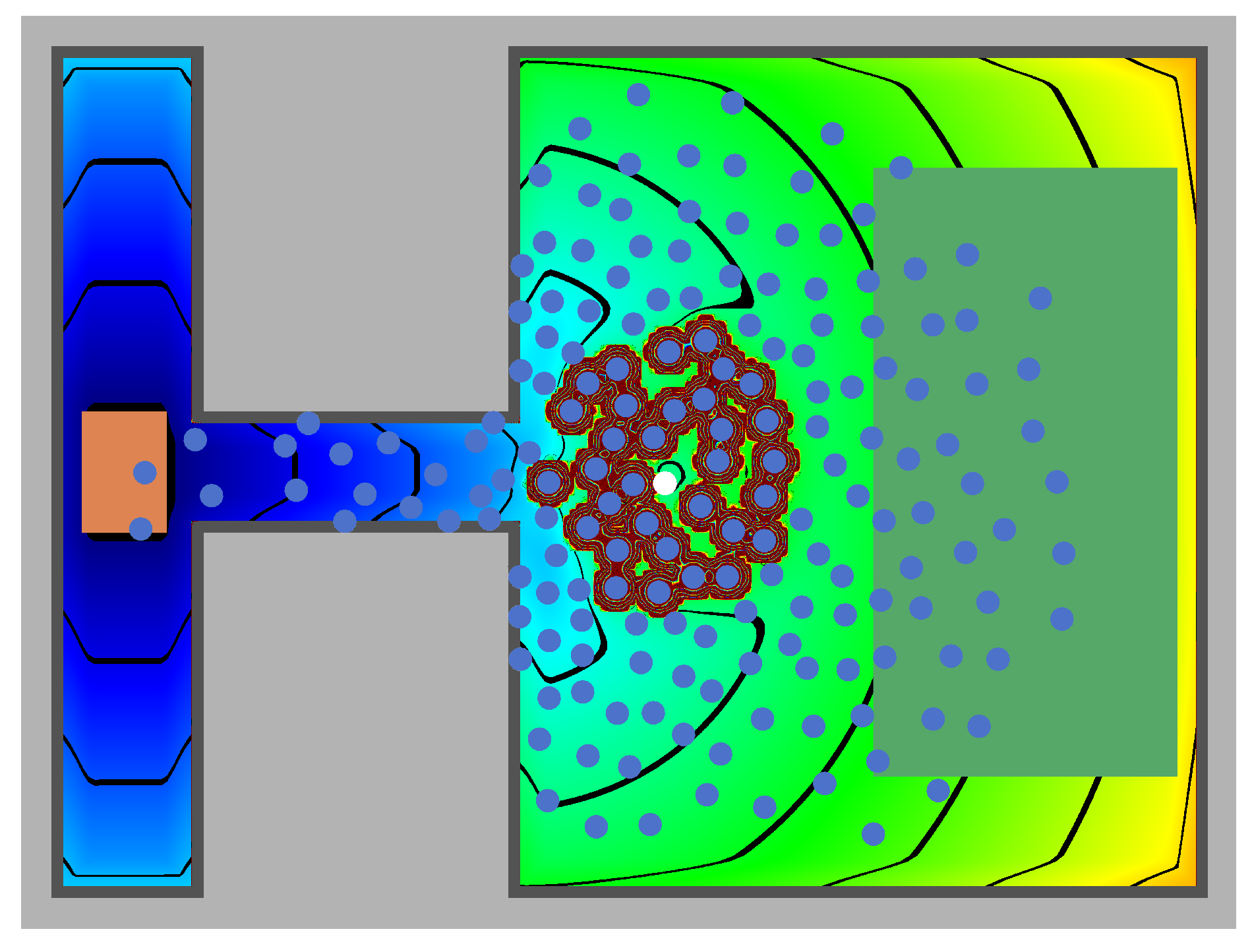
The full utility for an arbitrary agent in the bottleneck scenario is visualized in Figure 1. Agents that are regarded for the personal space utility of agent l can be identified by the strong gradient in the utility around them.
The target utility encodes the distance to the argent’s destination and can be interpreted as a cognitive map of the environment [13]. The distance to the destination is measured in the geodesic distance that considers obstacles, so that agents do not get stuck in more complex topographies. We solve the eikonal equation with the Fast Marching Method [38] to obtain the geodesic distances from all targets to every (grid) point in the topography.
While the floor field is calculated for the complete topography either once at the beginning of the simulation (static floor field) or at each simulation step (dynamic floor field) and belongs to a certain target or a list of targets that belong together, the combined utility belongs to agent l and it is only evaluated at current and prospective positions of agent l.
Each agent is assigned a personal space utility that represents pedestrians’ need for personal space in order to avoid collisions between agents. The implementation takes up the theory of (inter-) personal space by Hall [39], as described in [12]. Accordingly, the agent utility is divided into three parts, the intimate space—reserved for children and partners, the personal space, and the social space. More details can be found in Appendix A.1. Analogously, the behavior of agents around obstacles is handled by the utility function (see Appendix A.2).
Each agent in the simulation is assigned a free-flow speed. The free-flow speed is presumed to be the natural speed of an agent when the path is free. The agent accelerates to its free-flow speed if it moves unhindered through a free space. From the free-flow speed, a step length and step frequency are derived [11]. Based on the step frequency, steps of each agent are added to an event queue. This event queue enables a (pseudo-) continuous timeline. At a fixed rate, typically every , the accumulated events are processed in their order in the queue. For each event of an agent, the next position is calculated by maximizing the utility while using the Nelder–Mead method.
2.2. Bottleneck Scenario: Crucial for Improving Safety
Bottleneck scenarios are widely investigated in experiments [40,41,42,43,44] and simulations [45,46,47] within the pedestrian dynamics community, since constrictions can lead to increased densities and delays in evacuations. In addition, the flow through the bottleneck can be used for capacity estimation [42]. We recreate the setup of the experiments by Liddle et al. [41] in our crowd simulation tool Vadere [13].
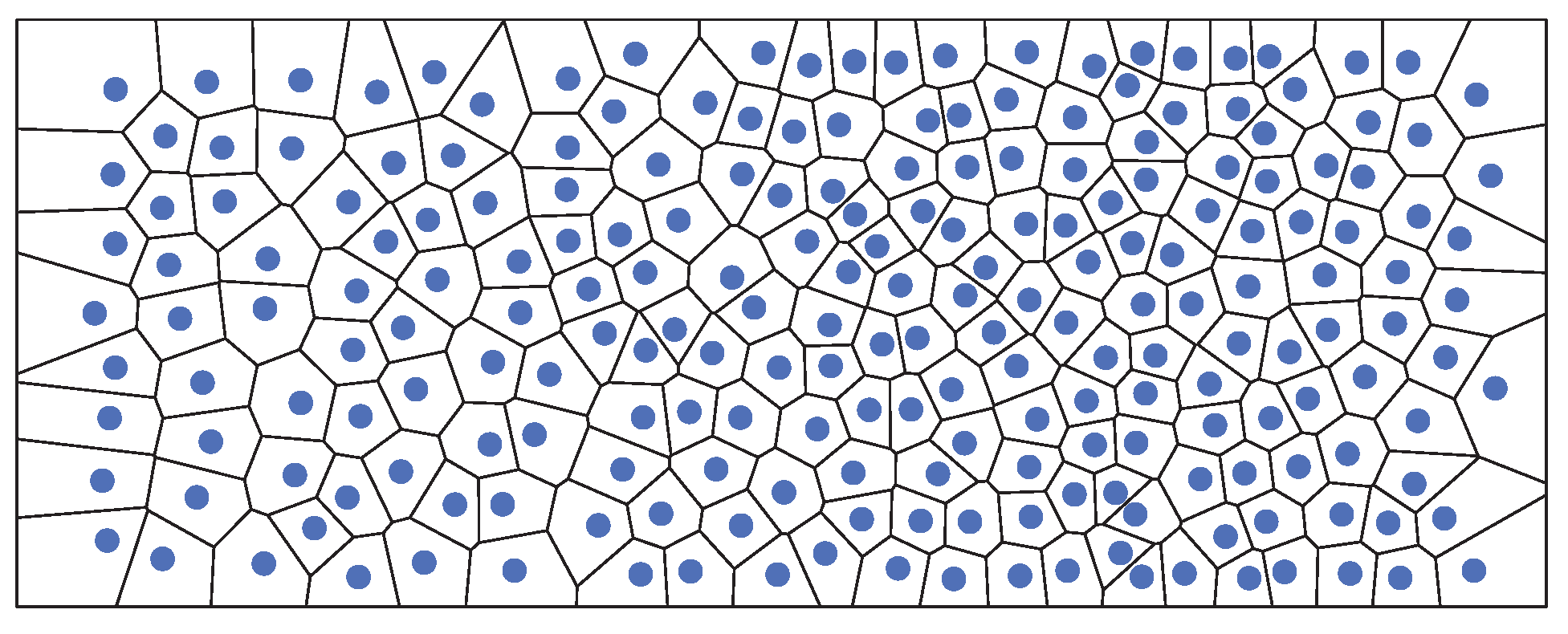
Our investigation of the bottleneck scenario focuses on the density in front of the bottleneck, similar to [41]. There are several ways to measure the pedestrian density. A common measure is Voronoi density [48,49], since it provides high accuracy and provides an output in number of agents per area, which is easy to understand. The Voronoi diagram identifies a Voronoi cell for each agent consisting of all points closer to this agent than to any other [49]. The density within the measurement area is calculated as the ratio between the number of agents in the measurement area to the sum of the areas of the Voronoi cells allocated to the agents within the area [11]. Figure 2 shows an exemplary Voronoi diagram. Agents who have more free space around them are assigned a larger Voronoi cell.
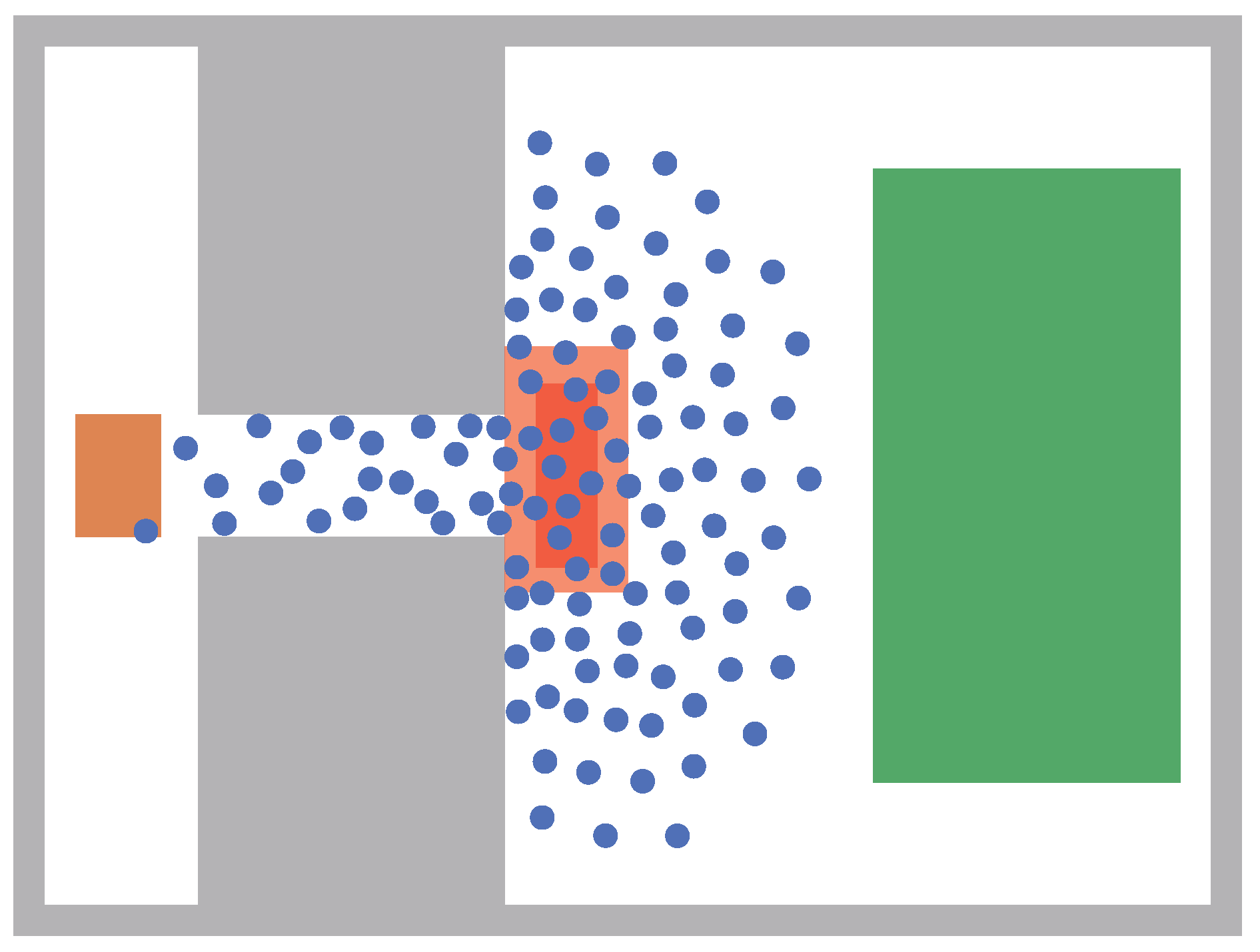
Figure 3 depicts a snapshot of the simulation at 30 s. In this setup, 220 agents (blue) are moving from their origin (green) through the bottleneck, which is constructed with obstacles (grey) to their destination (orange). In addition, two measurement areas are shown in front of the bottleneck (red). The density is calculated for the smaller area, the larger area is used for calculating the Voronoi diagram in order to avoid artifacts on the edge.
2.3. Choice of Sensitivity Analysis Methods
As discussed in the Introduction (Section 1.1), we are interested in a ranking of model parameters by their impact on the simulation outcomes to learn more about our models and, possibly, to reduce complexity. Variance-based approaches and, in particular, Sobol’ indices, have proved their worth in many applications ([18], p. 237ff). There are several open-source libraries for the approximation of Sobol’ indices due to their popularity. Furthermore, variance-based approaches need only model evaluations; gradients or further outputs are not necessary. Moreover, Sobol’ indices can be calculated as part of a forward propagation when using an approximation based on polynomial chaos [50] with reduced computational costs. All of these advantages make them an attractive choice for our application.
Variance-based methods serve to identify important parameters in the input parameter space. Based on the results, single parameters that were classified non-influential can be fixed to an arbitrary value within the range. This procedure is typically referred to as factor fixing. However, the analysis of parameter importance by itself may not point out enough potential for model reduction. Therefore, we also aim to identify important directions, which is, linear combinations of the input parameters that are particularly relevant. For this, we harness the theory of active subspaces [19,51]. Constantine and Diaz [26] also define activity scores as a sensitivity metric on single parameters that, in many situations, are similar to other sensitivity metrics, such as Sobol’ indices. Note that they are less versatile than Sobol’ indices, because they require (approximations of) model gradients. Generally, gradients are not directly available for most quantities of interest in locomotion models, even for differential equation-based models. In the case of the Optimal Steps Model, we approximate gradients through finite differences.
In this contribution, we combine all three aspects: we compute Sobol’ indices as a robust and dependable single-parameter sensitivity metric. They serve as reference for the activity scores, where we need to assure that the approximation of the gradients is sufficiently accurate. Finally, we identify an active subspace of important parameter directions.
From now on, the following nomenclature is used: we study a model that depends on a set of n input parameters . The output of the model is our quantity of interest. Both of the methods require a scalar simulation output.
2.3.1. Sobol’ Indices (Variance-Based Method)
For the description of Sobol’ indices, we assume that our model f is a square-integrable function defined over a k-dimensional unit hypercube . This description follows [52]. Any model that fulfills these assumptions can be represented by an analysis of variance, or ANOVA, decomposition. The decomposition splits f into a set of orthogonal functions, depending on the factors and their interactions:
First-order univariate functions represent independent contributions due to the individual parameters. Interaction terms to quantify the interactions of several input parameters on the response y. When all terms are used, the decomposition is an exact representation of f.
Sobol’ indices are a measure related to the variance of the model response y. This variance can be split into the variance of the functions in (2). Subsequently, the total variance of the response y can be written as
with . First order indices and total order indices are defined as
where . First order indices describe the variance in the response due to the variance in input parameter . In contrast to first order indices that only consider the effects of a single parameter, total order indices also consider interaction effects among parameters. The relation between the total order indices and the first and higher order indices is:
The total index for parameter i is the sum over all indices that contain a contribution of . The interaction effects can also be measured by the higher order indices defined by Sobol’. Total indices measure the variability of the output if all parameters, except , could be fixed.
For most problems in practice, these indices cannot be analytically calculated, since they require solving high-dimensional integrals. Instead, we approximate the Sobol’ indices by Jansen’s method [53]. For a given sampling factor M, the number of Monte Carlo samples generated is . We generate two matrices, A and B, with N samples each according to the input parameter density. The variation of all input factors except one is modeled by constructing matrices that are identical to matrix A, except for column i, which originates from matrix B. Subsequently, variances of model evaluations at row j of A and B to , respectively, are approximated. The first order indices are approximated by
where the variance of the model response is approximated by the sample variance of the evaluations and the subscript j stands for row j of the matrix. The total order indices are approximated by
2.3.2. Activity Scores (Derivative-Based Method)
The main idea of active subspaces [19] is to identify important parameter directions, which can be any linear combination of the input parameters. While they were originally designed for model reduction, Constantine and Diaz [26] suggest a way to use the interim results of this process to perform a global sensitivity analysis. The method described by Constantine et al. [19] is based on gradients. Central to the method is the calculation of the matrix
which is described as “(uncentered) covariance matrix of the gradient” ([51], p. 22) with input parameter density .
In practice, these high-dimensional integrals can neither be computed analytically nor by numerical quadrature and, therefore, C is typically approximated with a Monte Carlo approach while using M samples which are drawn :
We refer to the approximations by adding a hat () to the variable names. From now on, we describe the computation of the active subspaces and activity scores while using instead of C. The steps are identical for the true matrix C. We approximate the gradients by central finite difference quotients. Entry of the gradient is then calculated as
with step size h. In the next step, the eigenvalues of are analyzed using a spectral decomposition of the matrix:
A spectral gap in the eigenvalues identifies an active subspace: the largest gap separates the eigenvalues in two groups. We use the largest gap among the logarithmic representation of the eigenvalues. The eigenvectors associated with the first k eigenvalues above the eigenvalue gap form the active subspace . The remaining eigenvectors form the inactive subspace . If C is approximated by , Constantine shows that the distance between true and estimated subspace depends on the size of the spectral gap ([51], p. 54).
The i-th activity score [26] is calculated by summing over the k active eigenvalues multiplied with the squared entries of the i-th eigenvector:
Consequently, the activity scores depend on the user’s choice where to settle the eigenvalue gap therefore on the resulting size of the subspace k. While the largest gap in the eigenvalues should be used in theory, there might not always be a clear gap or only a certain size of subspace may be feasible.
2.4. Implementation of the Methods
We implemented both the approximation of activity scores and the approximation of the Sobol’ indices in Python. The scripts are available at https://github.com/pedestrian-dynamics-HM/mdpi-2020-vadere-sensitivity-analysis. The code is tested by comparison with the Ishigami function [54]. In addition, the results for the circuit model are reproduced and compare to [26]. Moreover, the results for the quadratic model from ([51], p. 38ff) are tested. Furthermore, unit tests, for example, for the approximation of the gradients have been implemented.
3. Results and Discussion
In this section, we first describe the setup of our sensitivity study, that is, the parameters we study, and how we run the crowd simulations. Next, we briefly show the impact of the parameters on the quantity of interest by analyzing scatterplots. Subsequently, we present and compare results of sensitivity analyses with first Jansen’s method for Sobol’ indices [52,53] and the active subspace method with corresponding activity scores [26].
3.1. Configuration of the Simulation
In contrast to many other applications, the initialization of a crowd simulation is typically stochastic, at least in parts. This is also the case for the Optimal Steps Model.
With the simulation start, agents are created and assigned a random free-flow speed and starting position. The free-flow speeds are drawn from a truncated normal distribution, the starting positions from a two-dimensional uniform distribution to cover a so-called origin area.
Consequently, different simulation runs lead to different results, unless the seed of the pseudo-random generator is fixed. Since positions and speeds are indeed unknown and do vary, fixing the seed would unduly simplify the model. This confronts us with a problem because the methods for sensitivity analysis presuppose deterministic outcomes. We adopt a pragmatic approach and use an average over 10 simulation runs for our quantity of interest. This has been successfully applied in [55] for occupant-evacuation time curves.
3.2. Uncertain Input Parameters in the Bottleneck Scenario
As briefly introduced in Section 2.2, we investigate a bottleneck scenario that is shown in Figure 3.
We choose six uncertain parameters that are listed in Table 1. The first two, mean and standard deviation of the free-flow speed, refer to the truncated Gaussian distribution from which the free-flow speeds are drawn. Note that truncating the normal distribution means that the two parameters are not independent. Because the goal of our contribution is rather a proof of concept for a valuable methodology than an in-depth analysis of queuing behavior at a bottleneck, we decided to treat them as independent parameters. In the simulation, the free-flow speed of an agent is also used to derive a dependent parameter [11], the individual step size of each agent. As third parameter, we vary the number of agents between 160 and 200. Typically, bottleneck experiments in experimental pedestrian dynamics study the effect of door widths on the density in front of the opening. Thus, we also vary the bottleneck width. Lastly, we vary a parameter that corresponds to each agent’s need for personal space, or distance to others: it is coded in the parameter of a function that expresses the utility of a position for an agent. See Appendix A.1 for more details on .
We want to point out that the parameters are of different character. Free-flow speed as well as personal space are properties of the agents, while the other two parameters, bottleneck width and number of agents, are parameters of the topography. It is important to keep this in mind when choosing the ranges for the parameters: Changes to topography parameters might change the dynamics of the system. Consequently, in our study, we had to make sure that within our parameter limits we maintain a bottleneck dynamic, that is, congestion in front of the constriction.
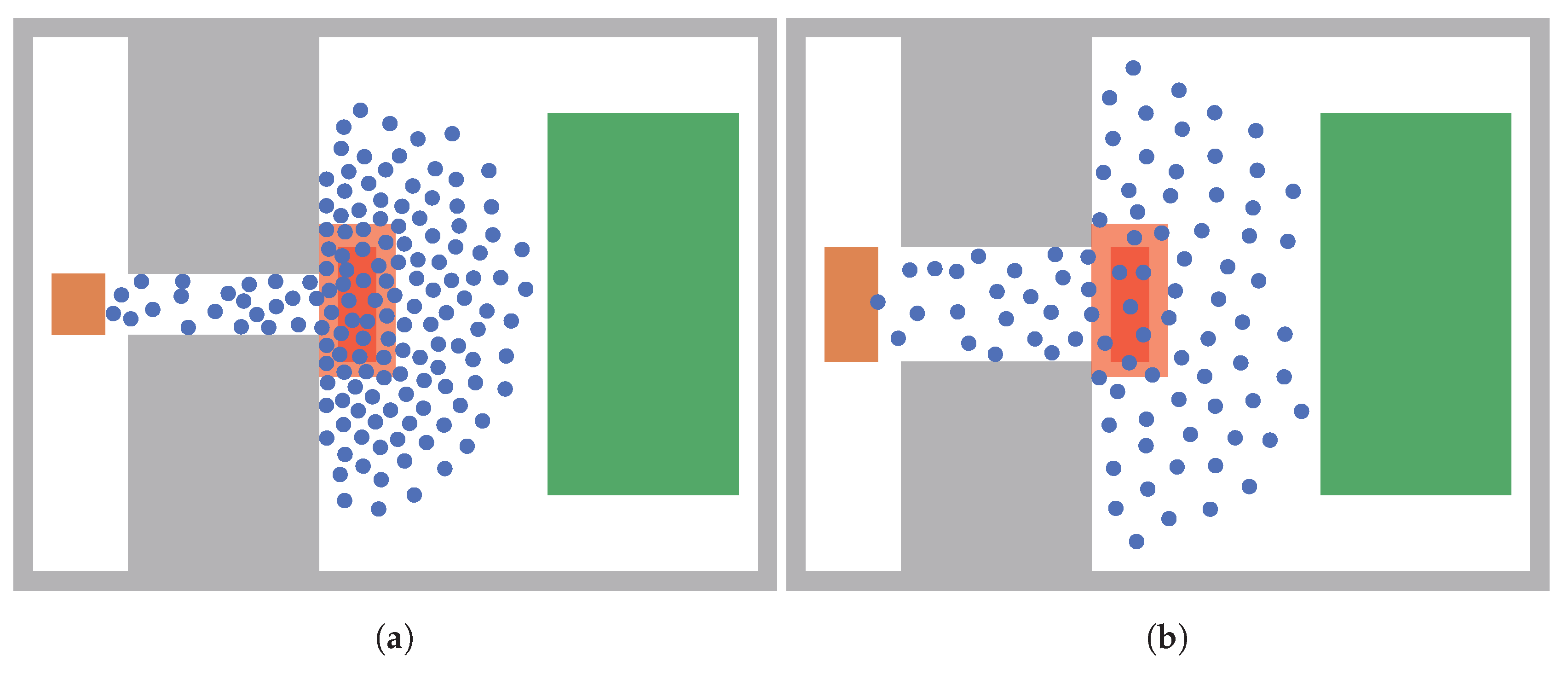
Figure 4 shows snapshots of the simulation of the bottleneck scenario. On the left, the lower limits of all parameters are chosen, on the right the upper limits of all parameters are chosen. The topography changes with the bottleneck width.
Because we study the feasibility of the methods in crowd simulation, we add a control parameter that is not actively used in the configuration of the simulation. We test whether the methods correctly detect the absence of an impact. Through the remaining "impact" of the control parameter, we also gain a measure for the inaccuracy that is caused by averaging several simulations. This procedure increases the number of evaluations and, therefore, the computation time, substantially. Hence, while a control parameter might be desirable, in principle, it will be out of question in computationally more demanding scenarios.
3.3. Relation between Parameter and Quantity of Interest
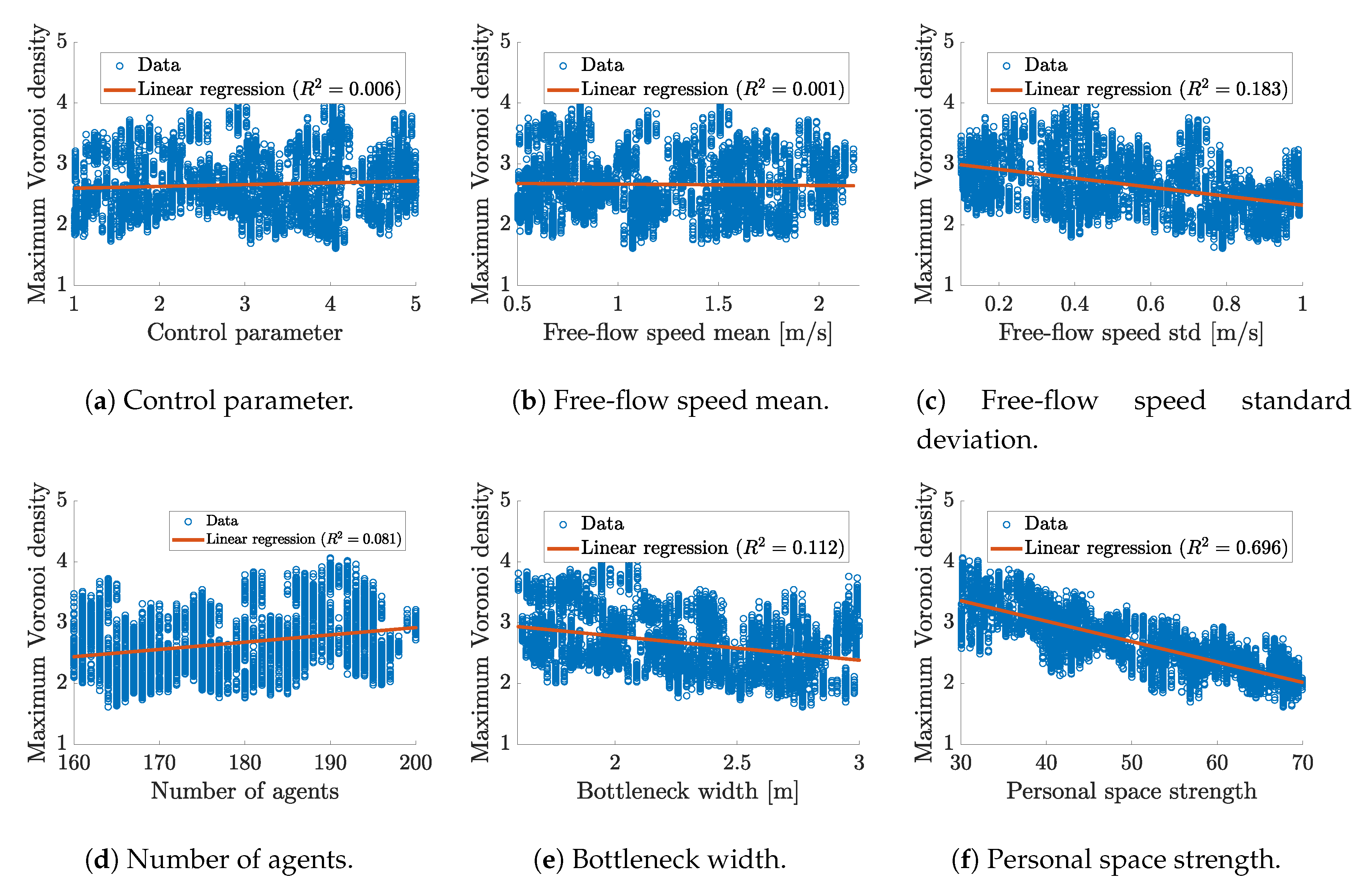
A starting point for a sensitivity analysis is to look at scatterplots between each input parameter and the quantity of interest, according to ([23], p. 113). Our quantity of interest is the crowd density in front of the opening, more precisely the maximum Voronoi density that is described in Section 2.2, measured in persons per square meter. We use the maximum of the Voronoi density over simulation time in order to obtain a scalar quantity of interest. Figure 5 shows the scatterplots. Please note that all parameters are varied at the same time. Each scatterplot shows a projection for the parameter that is shown on the horizontal axis.
There is only one parameter with a clear correlation to the maximum Voronoi density: the strength of the need for personal space. As expected, a more pronounced need for personal space results in a lower density in the front of the bottleneck, where our measurement area is placed. In addition, we observe a slight trend for the bottleneck width. The density decreases with a wider opening. For the other three parameters, there is no clear trend visible, their responses are similar to the control parameter’s response.
In summary, the scatterplots indicate a strong impact of the need for personal space and a medium impact of the bottleneck width on the maximum Voronoi density. The other parameters do not seem to have a clear individual impact. However, interaction terms among them might have a strong impact. To identify higher order relations, we study the sensitivities in more detail with Sobol’ indices and activity scores. Note that the choice of the quantity of interest has an impact on the strength of the correlation between input parameters and the simulation outcome. Therefore, it is important to choose a quantity of interest tailored to the research question of the study.
3.4. Sobol’ First and Total Order Indices
We approximate Sobol’ total and first order indices with Jansen’s method [53]. The variance-based approach of this metric is suited for most models, since it requires only model evaluations. Nevertheless, a high number of model evaluations is typically required.
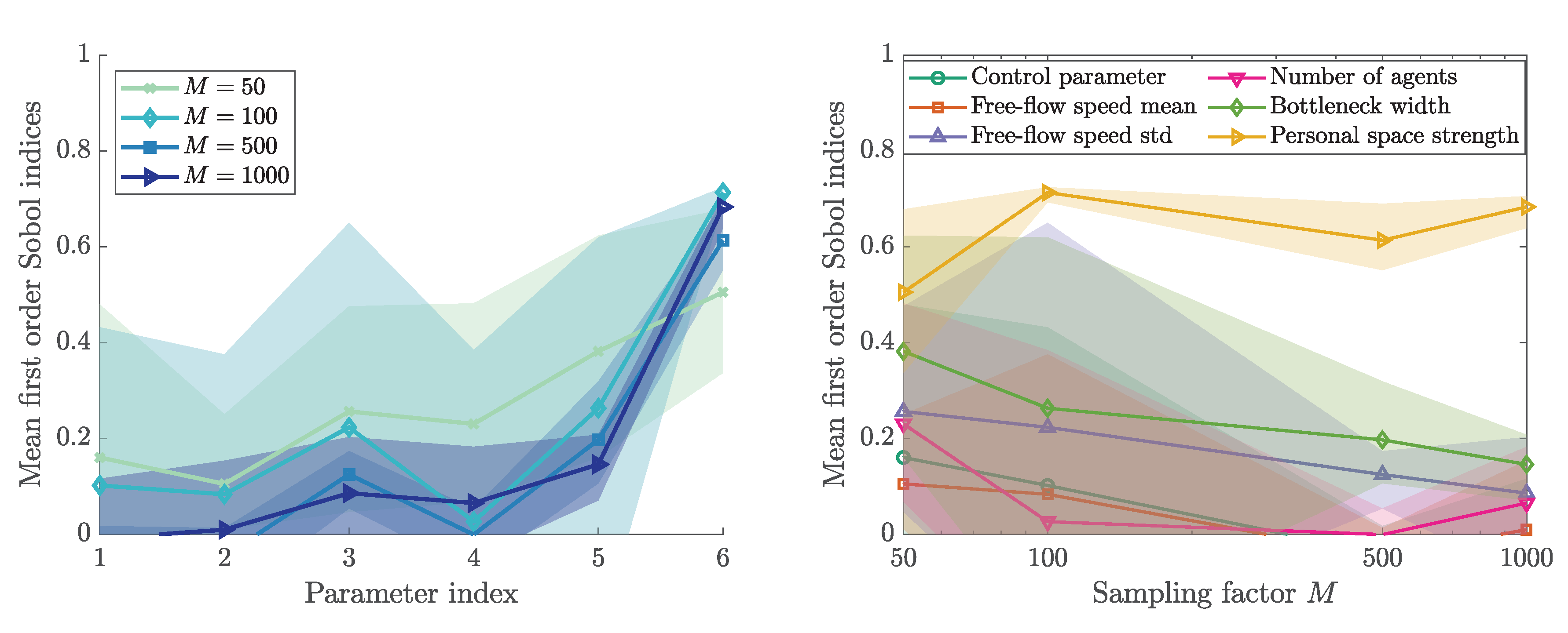
Figure 6 depicts the first order indices for the bottleneck scenario. The first order index describes the variance in the output stemming solely from parameter i. The negative indices are due to numerical errors, a commonly observed issue especially with a small sample size [52]. We can observe fewer negative entries with larger M, which is larger sample sizes.
We observe a high influence by the bottleneck width. In addition, we observe the lowest variation between the runs for this parameter. The indices reflect that the control parameter has no impact on the quantity of interest. In addition, the mean free-flow speed as well the number of agents do not have a measurable individual impact on the density in front of the bottleneck. However, they might be influential in interaction terms. Therefore, we investigate the total order indices next.
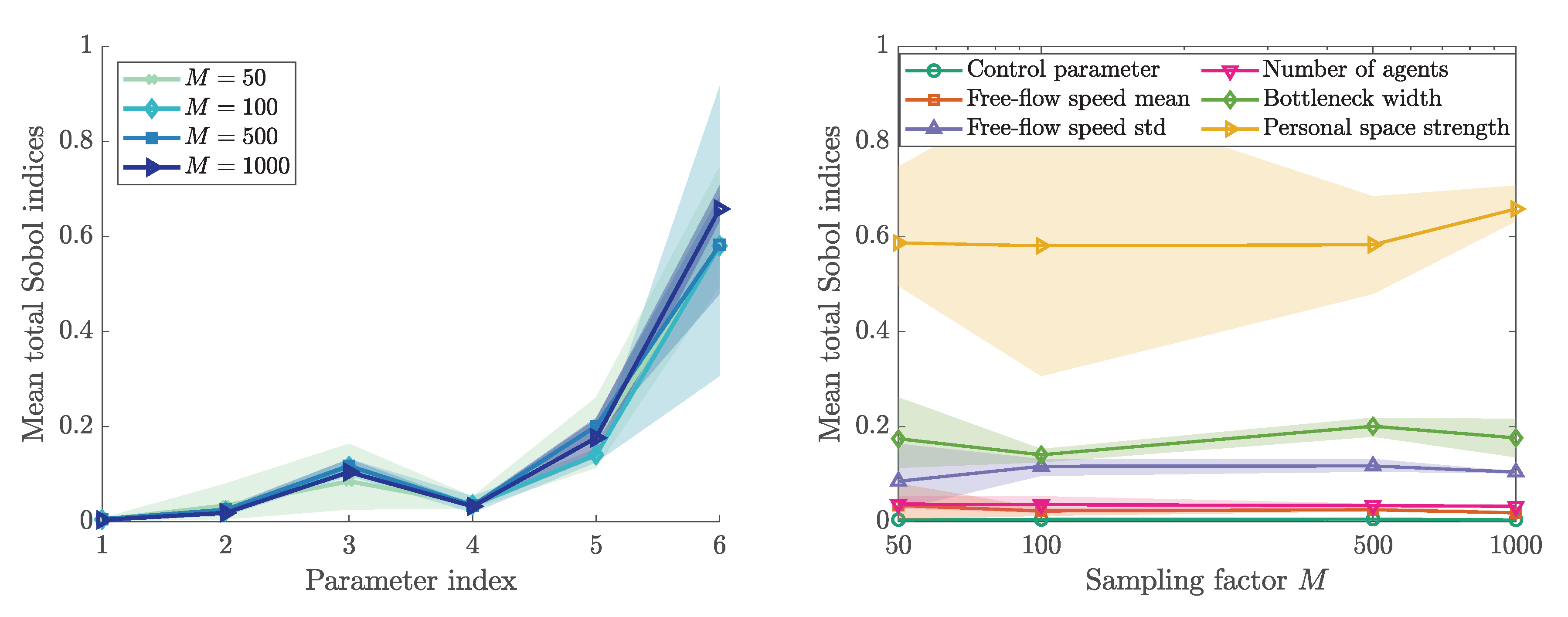
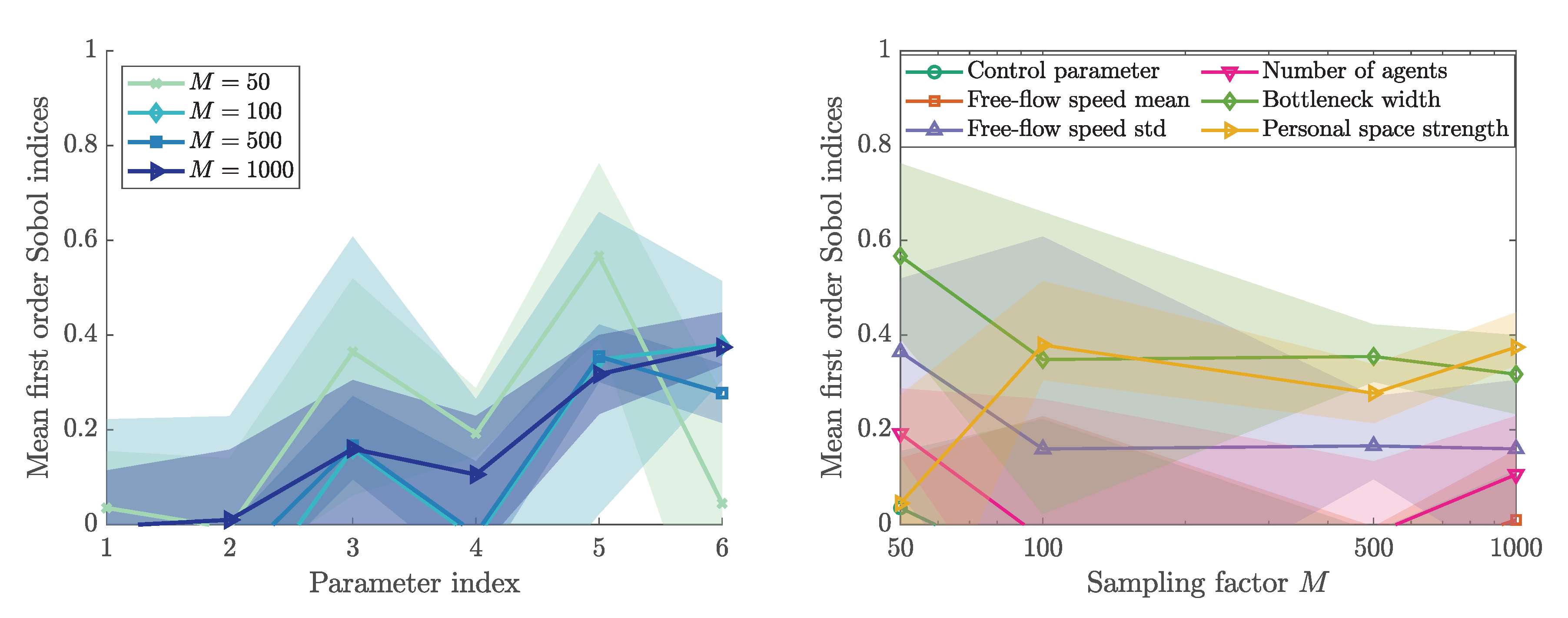
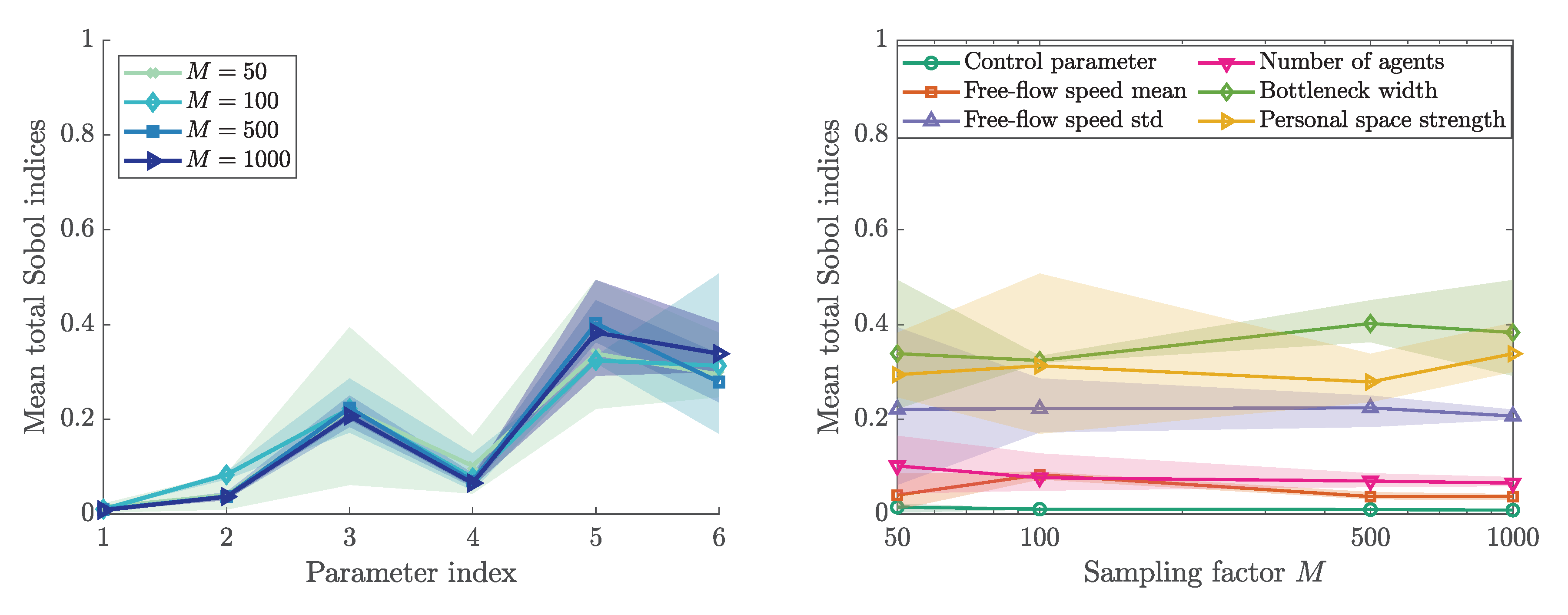
In addition, Figure 7 plots Sobol’ total indices. The sum of the first order indices is almost identical to the sum of the total order indices. That means there are no strong interactions among the factors, compare (5). The number of samples for the matrices A and B for Jansen’s method are defined by . For each sampling factor M, three runs are performed in order to study the variation in the results. The average (solid lines) is shown together with the extremes (area). As expected, the variation decreases with an increasing number of samples. From the total indices, we can conclude that the first (control parameter), second (free-flow speed mean), and fourth (number of agents) parameter are non-influential. The personal space strength (parameter index 6) is the most influential parameter.
3.5. First Eigenvector and Activity Scores
When looking for active subspaces in crowd simulations, it is important to keep in mind that the method cannot be used for purely rule-based models where the concept of gradients is meaningless. This especially applies for cellular automaton models. For most other models, as for the Optimal Steps Model used here, gradients for the quantity of interest may not be directly available, but they can be approximated. We use central difference quotients for this.
According to [26], we normalize each input parameter to the interval . For each parameter, the step-size h for the central difference is scaled by the parameter’s range. We choose the smallest possible step size for h: since the number of agents is a natural number, h has to scale to at least one agent. Based on the range of the parameter “number of agents”, the step size is set to . All of the sensitivity results are presented for the normalized model.
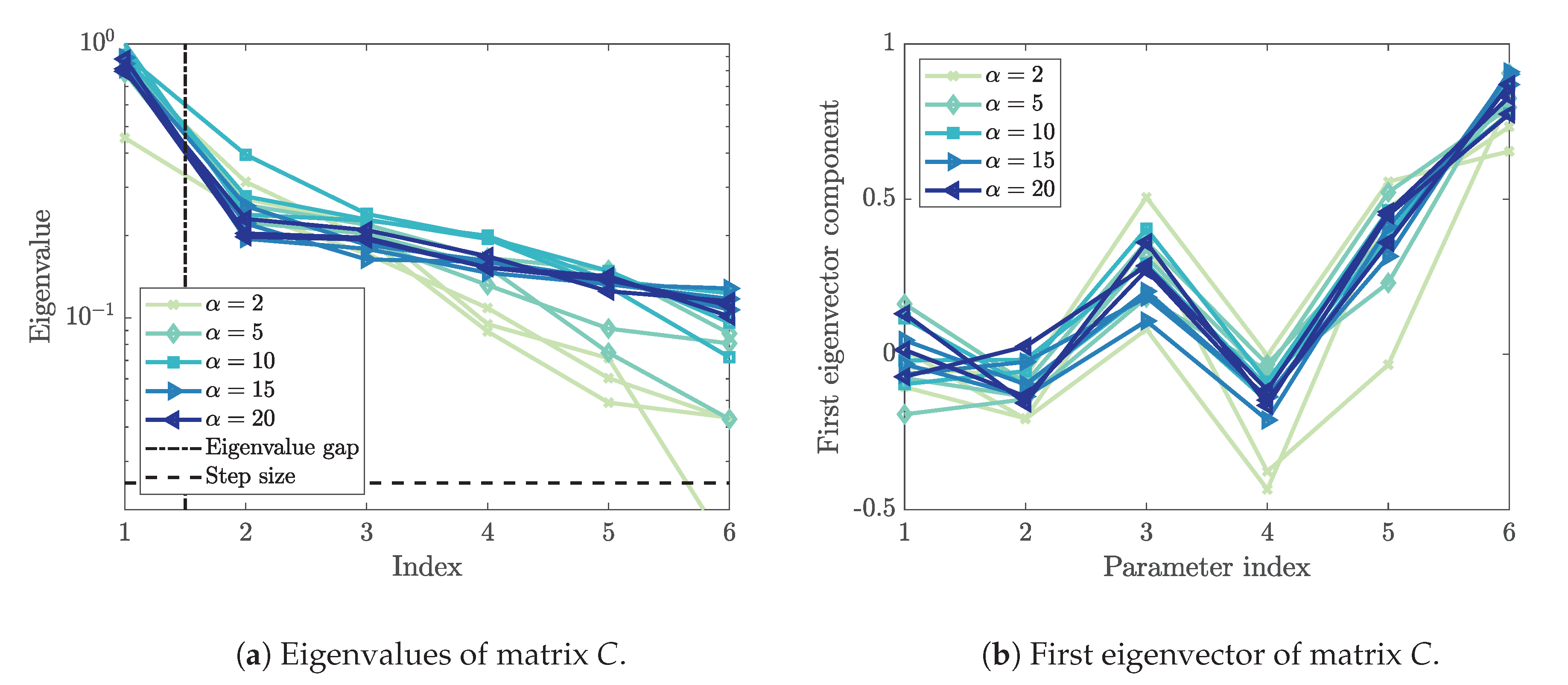
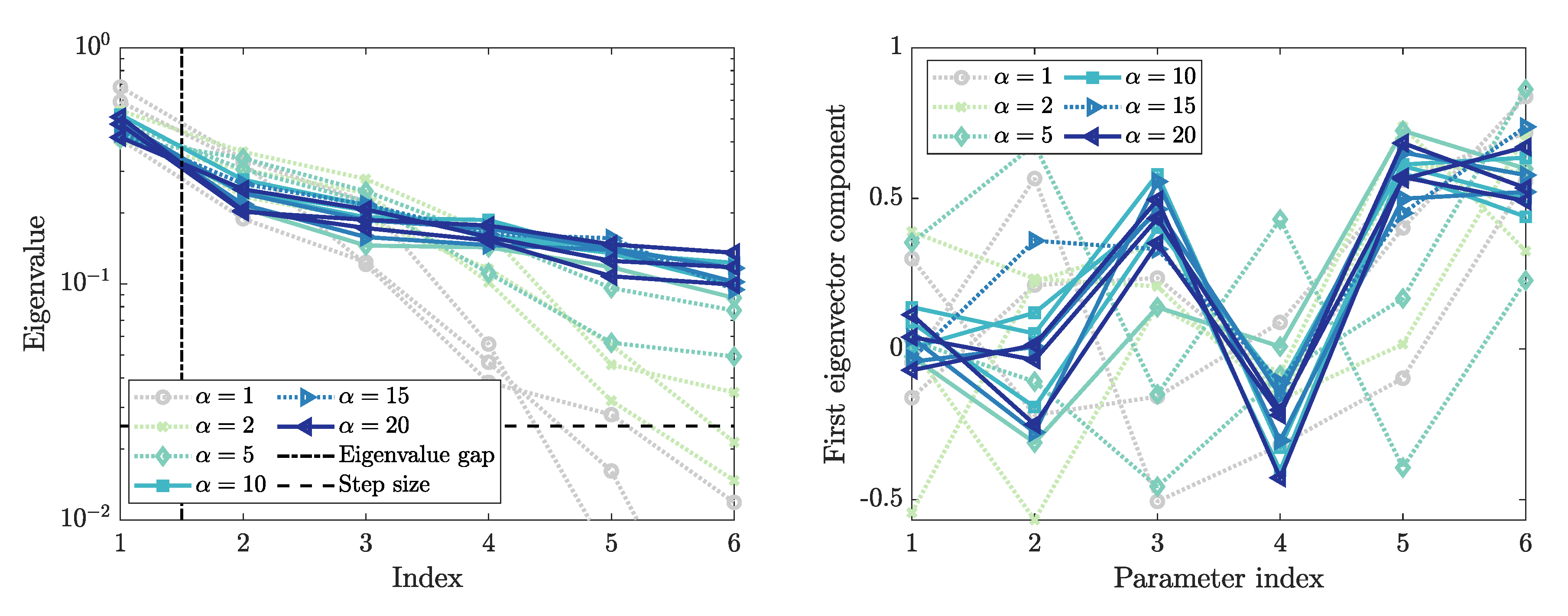
Figure 8a presents the eigenvalues of the matrix , obtained from the gradient samples according to (9). A spectral gap is present between the first and second eigenvalue. That means we identify a one-dimensional active subspace defined by the first eigenvector. Since the gap is clearly above the chosen step size (including the first eigenvalue below the gap), we can assume that the gap is real and not based on a phantom eigenvalue. The first eigenvector is shown in Figure 8b. From the scatterplots in Figure 5, we know that the personal space strength correlates negatively with the maximum Voronoi density. Accordingly, we rotate the first eigenvector. Now, the first eigenvector entries show the direction in which each parameter contributes to the quantity of interest. The standard deviation of the free-flow speed, bottleneck width, and personal space strength have a negative impact on the outcome. That means, if these parameters are increased, a reduced (maximum Voronoi) density will be observed. The first eigenvector is the most dominant parameter direction in the input parameter space.
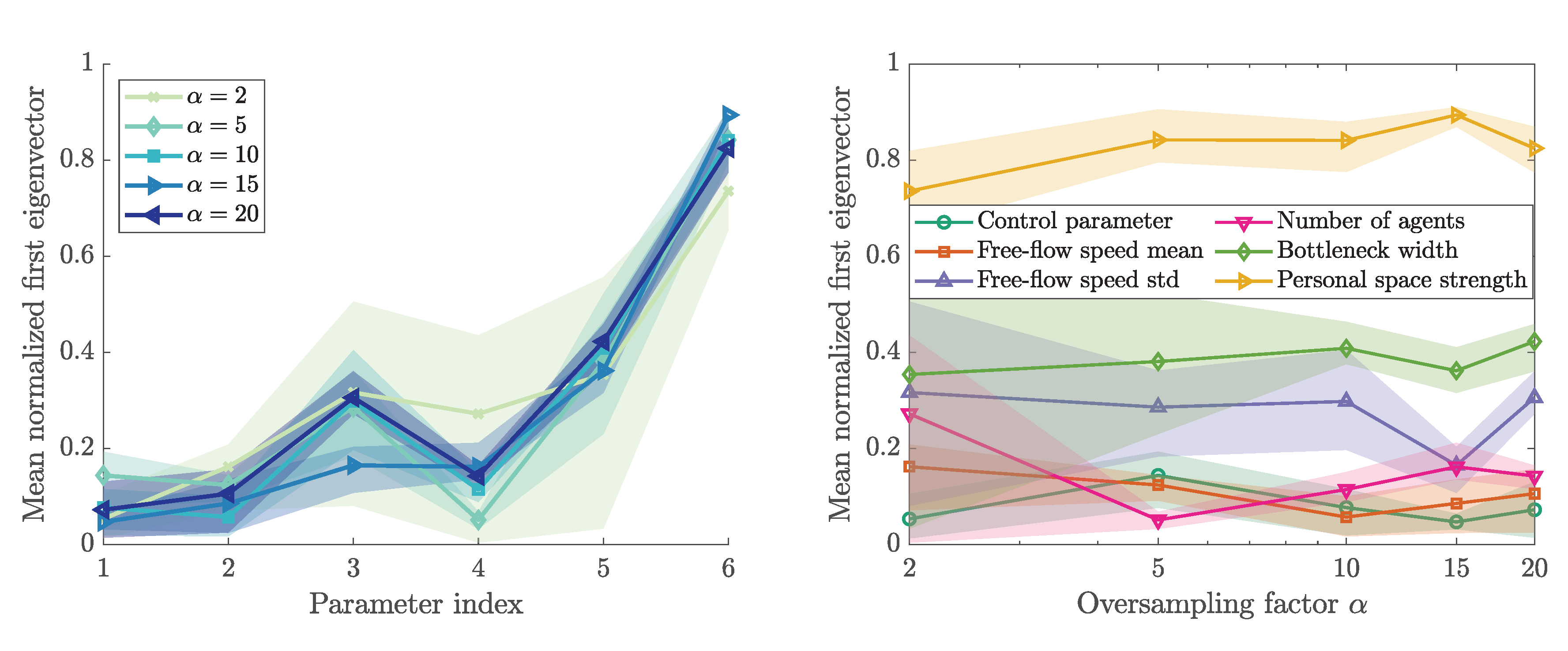
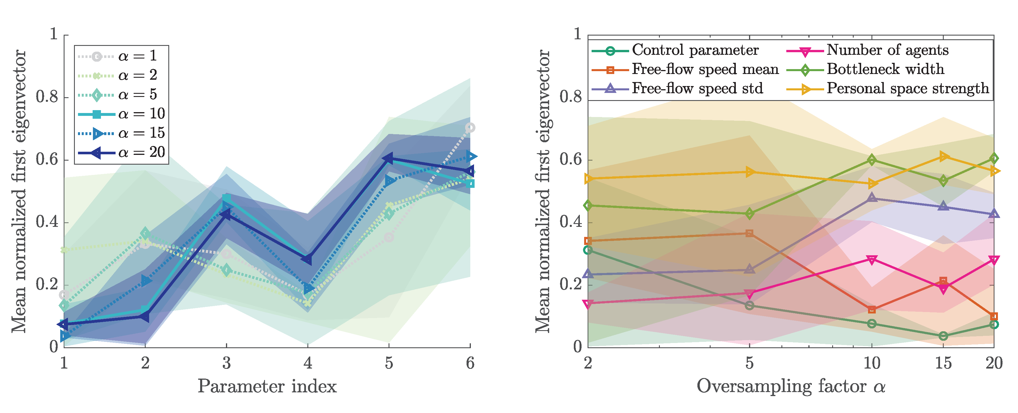
Independent of the size of the active subspace, the first eigenvector entries also constitute a sensitivity metric. Therefore, we normalized the absolute first eigenvector according to [26] by the length of the vector. The resulting measures are shown in Figure 9.
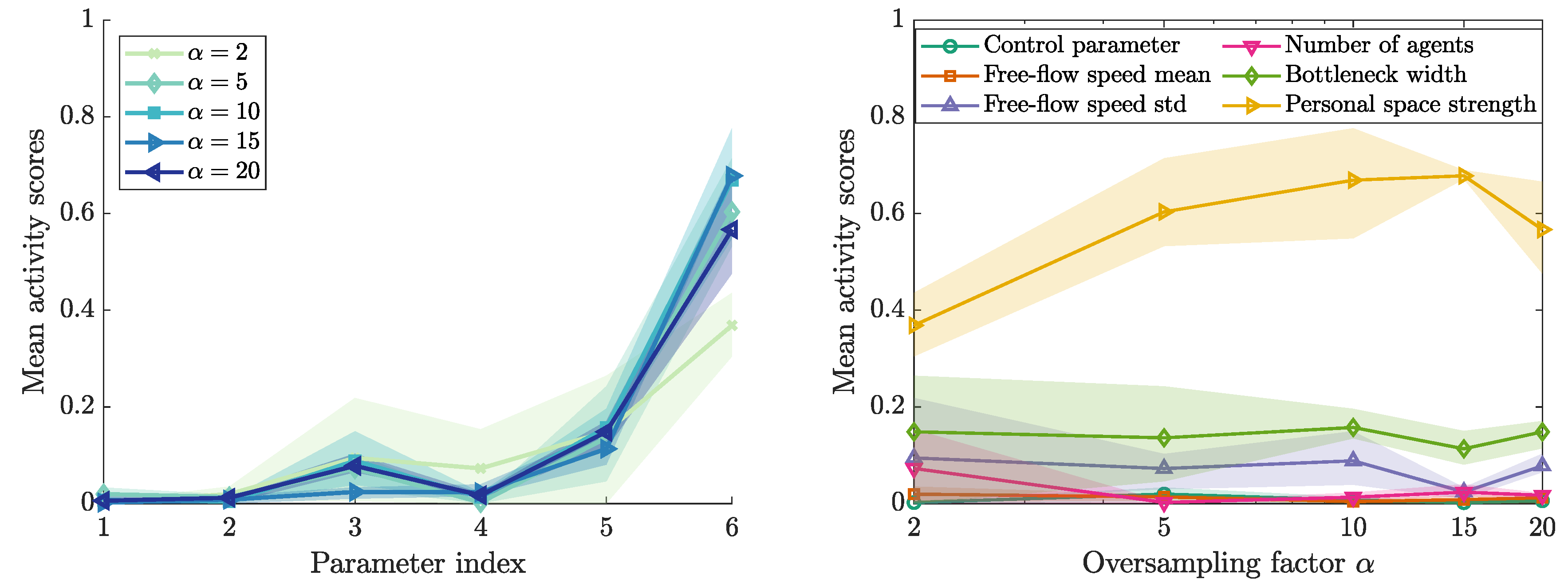
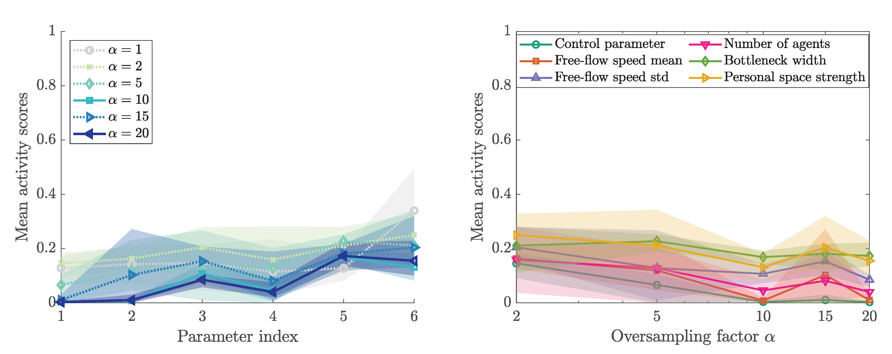
From the active subspace we identified, we can now derive the activity scores while using (12). Figure 10 presents the activity scores for different oversampling factors . The oversampling factor determines the number of gradient samples used for the approximation of C: . Here, m is the number of parameters and is the expected size of the subspace. According to ([51], p. 35), M evaluations of the gradient approximate the first k eigenvalues of C sufficiently accurate. The oversampling factor is typically chosen between 2 and 10 ([51], p.35). As expected, the variation of the activity scores for a fixed oversampling factor, represented by the area around the mean, diminishes with larger oversampling factors. In accordance with the first eigenvector metric, the personal space strength is clearly the most influential parameter. The method recovers a small activity score for the control parameter. We use this value as a threshold that a parameter must exceed in order to be considered influential. Two other parameters, the mean of the free-flow speed and the number of agents seem to fail that criterion, and, thus, are deemed non-influential.
The one-dimensional subspace can be used to construct a surrogate model for our original model with a lower-dimensional input parameter space, in our case, a one-dimensional input space.
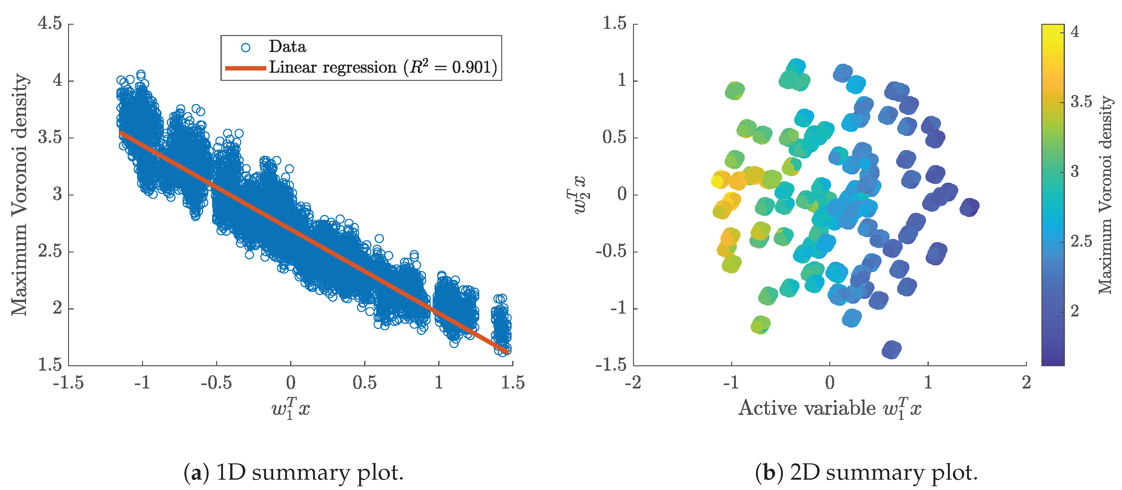
Any input parameter vector can be projected onto this subspace by the active subspace , here, just the first eigenvector . The transformation of a parameter vector x in the active subspace yield the corresponding value of the so-called active variable . Figure 11 shows the sufficient summary plots: the one-dimensional sufficient summary plot depicts the quantity of interest against the active variable. The linear regression reveals a strong correlation between input and output. The coefficient of determination is significantly higher than for each single parameter, compare Figure 5. The two-dimensional summary plot shows the active variable against the inactive variable . is the highest ranked eigenvector of the inactive subspace, i.e., this parameter direction has the largest impact among the direction in the inactive subspace. This plot confirms that the one-dimensional subspace is well chosen, since the change in the maximum Voronoi density (color coded) is mainly visible in the direction of the active variable of the one-dimensional subspace .
3.6. Sensitivity Ranking
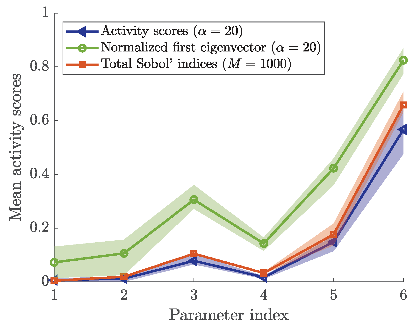
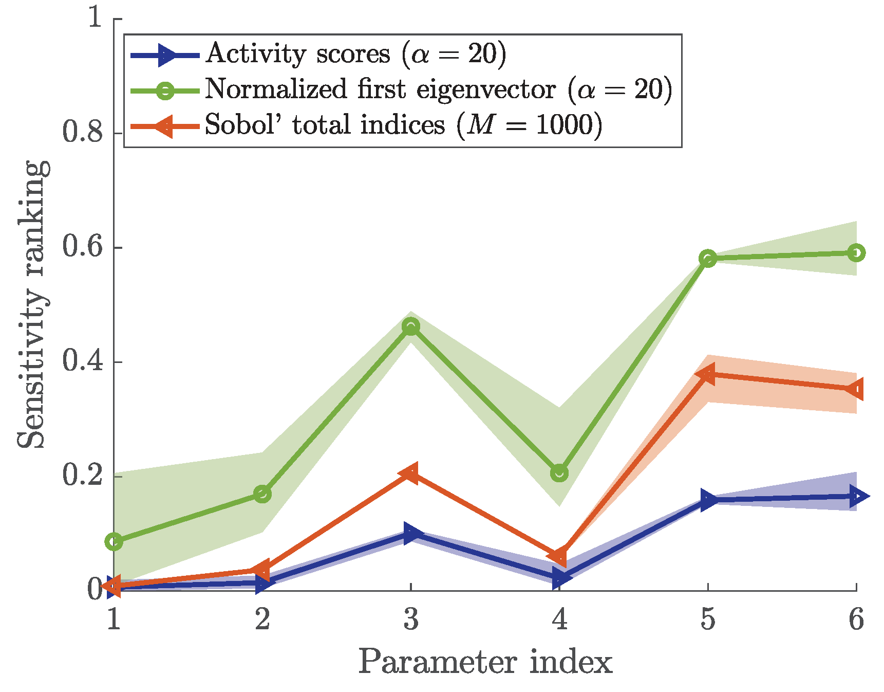
In Figure 12, we present the normalized indices for visual comparison. According to [26], we also show the first eigenvector as a sensitivity metric additionally to the Sobol’ indices and the activity scores. The parameters are ranked consistently for all three indices. In addition, Sobol’ indices and activity scores assign the control parameter a ranking that is close to zero, reflecting that it has no impact on the outcome.
The agreement between the results of both Sobol’ indices and activity scores support the hypothesis that activity scores with finite difference approximation of the gradients can be applied to crowd simulation, and more specifically the Optimal Steps Model.
All the metrics assign small indices with the control parameter. This indicates that they are able to recover that this parameter has no impact on the chosen quantity of interest. We use the non-zero sensitivity index assigned with the control parameter as indication: each parameter that is assigned an index smaller than the control parameter’s index is classified as a non-influential parameter. If the control parameter is assigned a sensitivity index of zero, a different threshold must be found. In our setup, the mean of the free-flow speed, as well as the number of agents are—within their respective ranges—non-influential for the maximum Voronoi density in front of the bottleneck. The most influential parameter is clearly the personal space strength. This is plausible because the mean free-flow speed is not directly related to the density, neither is the number of agents. If resources are available to determine uncertain factors (and it is possible), the personal space strength should be studied first in order to reduce the uncertainty in the prediction.
3.7. Impact of the Parameter Range
So far, all of the measures have shown that varying the personal space strength parameter over the interval has the largest impact on the maximum Voronoi density. However, the range of the personal space strength parameter is difficult to determine. First, it is a non-physical parameter, which means that we cannot measure it directly. Second, we know that personal space also depends on the society and on cultural effects [56]. Third, other factors, such as groups and social identities, will have an impact on the need for personal space [57].
In view of this complexity, we decided to run our analysis for a second, much smaller parameter interval. The changed parameter limits are listed in Table 2, all other parameter ranges are set as before, according to Table 1.
The result of the analysis is shown in Figure 13. We observe three effects: first, there is a larger variation between different runs—even for a high number of samples (for or , respectively). Appendix B contains the results with both methods. Second, the indices differ significantly from the indices obtained with the original parameter ranges, as shown in Figure 12, especially for the personal space strength parameter. Third, while the relative ranking of the parameters is still similar, there are larger differences between indices among the methods than for the original interval (Figure 12).
We conclude that a trustworthy sensitivity study of the personal space strength parameter requires a pre-calibration of the parameter to empirical data. However, while controlled experiments for the bottleneck exist, e.g., [41], they do not deal with psychological parameters. We argue that, in this case, the method helps to indicate a direction for future research. An approach to pre-calibration is discussed in Appendix B.3.
4. Conclusions
We studied the sensitivities of a set of input parameters in a simulation model of a fundamental scenario in pedestrian dynamics: a bottleneck. We looked at the crowd density in front of the opening as quantity of interest.
We used variance-based and derivative-based sensitivity measures. As a variance-based sensitivity metric, we chose Sobol’ first order and total indices. They purely rely on model evaluations. Both other measures, the first eigenvector and the so-called activity scores, stem from the active subspace ansatz. This approach is based on gradient evaluations that we approximated through central finite difference quotients.
The results of all measures coincided and thus confirmed each other. We were able to identify two of the input parameters as non-influential with respect to the quantity of interest: the mean free-flow speed and the number of agents. These parameters can be fixed for further studies, such as uncertainty analysis or model calibration to any value within the investigated range. It also supports the informative value of many controlled bottleneck experiments, where the number or participants was not or was hardly varied.
Most interestingly, we identified a one-dimensional active subspace in the input parameter space. That means a single linear combination of the input parameters shows a dominant correlation with the simulation results. The active subspace can be used to find a so-called ridge approximation, which is a surrogate model that is based on the important input parameter direction.
The sensitivity metrics were plausible: they agreed with our expectations in size and direction of their relationship with the quantity of interest. For our application, pedestrian dynamics, the results demonstrate that sensitivity metrics from uncertainty quantification are not only systematic and standardized, but also powerful tools to study parameter sensitivities. They point out non-influential and identity most influential parameters. Thus, they help with research prioritization, notably for empirical research.
Author Contributions
Conceptualization, R.F., M.G. and G.K.; methodology, M.G.; software, M.G.; validation, M.G.; formal analysis, M.G.; investigation, M.G.; resources, G.K.; data curation, M.G.; writing–original draft preparation, M.G.; writing–review and editing, R.F, M.G. and G.K.; visualization, M.G.; supervision, R.F. and G.K.; project administration, R.F., M.G. and G.K.; funding acquisition, G.K. All authors have read and agreed to the published version of the manuscript.
Funding
This research was funded by the German Federal Ministry of Education and Research grant numbers 13N14464 and 13N14562. This work was financially supported through the Open Access Publication fund of the Munich University of Applied Sciences.
Acknowledgments
The authors would like to thank Mario Teixeira Parente for discussions on active subspaces and activity scores. The authors acknowledge the support by the Faculty Graduate Center CeDoSIA of TUM Graduate School at Technical University of Munich and the research office FORWIN at Munich University of Applied Sciences.
Conflicts of Interest
The authors declare no conflict of interest.
Appendix A. Optimal Steps Model Utilities
The Optimal Steps Model is implemented in our open-source simulation framework Vadere, available at www.vadere.org. The utility functions are implemented in the package org.vadere.simulator.models.potential. Table A1 maps the symbols from the equations to the variable names in the implementation. In addition, the default parameter value defined in AttributesPotentialCompactSoftshell for each value is given. The radii of the personal and intimate space stem from Hall [39].

Table A1.
Mapping between the notation in the Vadere code and the mathematical description of the utility functions.
Table A1.
Mapping between the notation in the Vadere code and the mathematical description of the utility functions.
| Variable (Equation) | Variable (Code) | Default Value | Unit |
|---|---|---|---|
| intimateSpaceFactor | 1.2 | ||
| intimateSpacePower | 1 | ||
| personalSpacePower | 1 | ||
| pedPotentialPersonalSpaceWidth | 1.2 | m | |
| pedPotentialIntimateSpaceWidth | 0.45 | m | |
| pedPotentialHeight | 50.0 | ||
| obstPotentialHeight | 6.0 | ||
| obstPotentialWidth | 0.8 |
Appendix A.1. Agent Utility
To assure that agents keep a distance to other distance, we introduce the personal space utility. The model for the personal space utility can be written as [12,13]
with
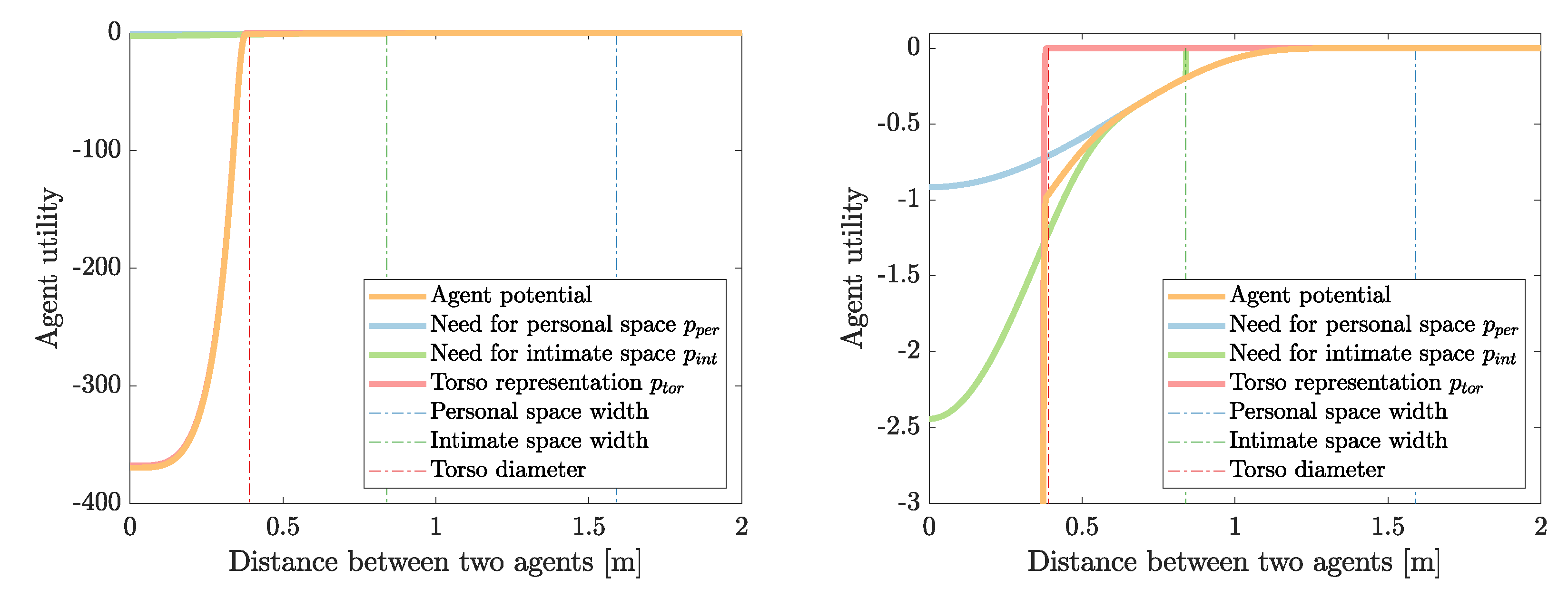
Here the radius of agent i’s torso and , are the radii of the personal and intimate space of agent l. is the Euclidean distance between the position of agent i and x of agent l, that is, . This model is implemented in PotentialFieldPedestrianCompactSoftshell. In the current implementation of the Optimal Steps Model, the personal spaces and radii of all agents are identical. This so-called soft-shell utility is depicted in Figure A1.
Figure A1.
Soft-shell agent utility models the personal and intimate space of agents.

Appendix A.2. Obstacle Utility
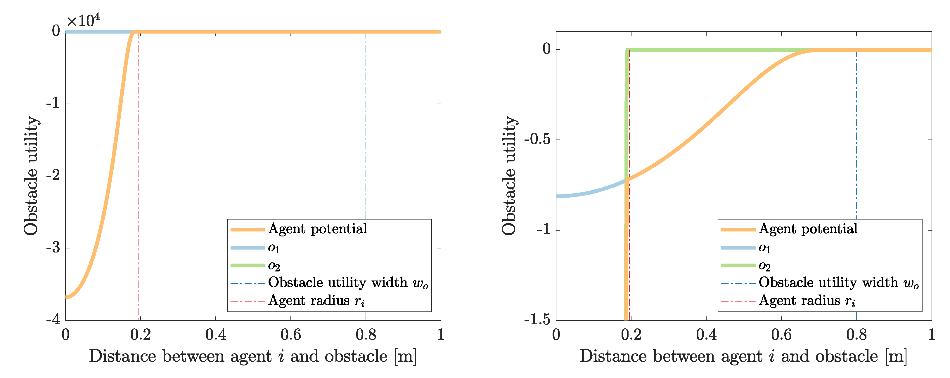
Additionally, to assure that agents are not colliding with obstacles an obstacle utility is defined. Since the floor field is not defined inside obstacles, agents cannot step on an obstacle. The obstacle utility models the natural behavior of pedestrians around obstacles: If there is enough space, pedestrians keep a distance from obstacles. The fewer space they have, the closer they might move towards the obstacle. The obstacle utility is implemented in PotentialFieldObstacleCompactSoftshell. It is based on the theory of Hall [39] and defined in [12] as:
with
where is the distance between position x and the closest point of the obstacle, and are the height and width of the obstacle utility, respectively, and is radius of agent i. The obstacle utility function is visualized in Figure A2.
Figure A2.
Soft-shell obstacle utility models the behavior of an agent around an obstacle.

Appendix B. Impact of Parameter Ranges
The full set of the adapted input parameters are shown in Table A2.
Table A2.
Uncertain parameters and their distribution used for the sensitivity analysis.
| Index | Parameter | Range | Type |
|---|---|---|---|
| 1 | Control parameter | float | |
| 2 | Free-flow speed mean [m/s] | float | |
| 3 | Free-flow speed std [m/s] | float | |
| 4 | Number of agents [1] | int | |
| 5 | Bottleneck width [m] | float | |
| 6 | Personal space strength [1] | float |
Appendix B.1. Sobol’ First and Total Order Indices
The first and total Sobol’ indices for the new range of the personal space strength parameter are shown in Figure A3 and Figure A4, respectively.
Figure A3.
First order Sobol’ indices for the new range of the personal space strength parameter. The parameter index is mapped as follows: 1—control parameter, 2—free-flow speed mean, 3—free-flow speed standard deviation, 4—number of agents, 5—bottleneck width, 6—personal space strength.
Figure A3.
First order Sobol’ indices for the new range of the personal space strength parameter. The parameter index is mapped as follows: 1—control parameter, 2—free-flow speed mean, 3—free-flow speed standard deviation, 4—number of agents, 5—bottleneck width, 6—personal space strength.

Figure A4.
Total order Sobol’ indices for the new range of the personal space strength parameter. The parameter index is mapped as follows: 1—control parameter, 2—free-flow speed mean, 3—free-flow speed standard deviation, 4—number of agents, 5—bottleneck width, 6—personal space strength.
Figure A4.
Total order Sobol’ indices for the new range of the personal space strength parameter. The parameter index is mapped as follows: 1—control parameter, 2—free-flow speed mean, 3—free-flow speed standard deviation, 4—number of agents, 5—bottleneck width, 6—personal space strength.

Appendix B.2. First Eigenvector and Activity Scores
Figure A5 depicts the activity scores for the updated limits on the personal space strength parameter. In addition, the first eigenvector metric is shown in Figure A6. The eigenvalues and first eigenvector of the matrix C are presented in Figure A7.
Figure A5.
Activity scores for the new range of the personal space strength parameter. Runs that identify a one-dimensional subspace are shown with solid lines, in some runs a 5-dimensional subspace is identified (dotted). The parameter index is mapped as follows: 1—control parameter, 2—free-flow speed mean, 3—free-flow speed standard deviation, 4—number of agents, 5—bottleneck width, 6—personal space strength.

Figure A6.
Normalized first eigenvector metric for the new range of the personal space strength parameter. Runs that identify a one-dimensional subspace are shown with solid lines, in some runs a higher dimensional subspace is identified (dotted). The parameter index is mapped as follows: 1—control parameter, 2—free-flow speed mean, 3—free-flow speed standard deviation, 4—number of agents, 5—bottleneck width, 6—-personal space strength.

Figure A7.
Eigenvalues and first eigenvector of the matrix C for the new range of the personal space strength parameter. Runs that identify a one-dimensional subspace are shown with solid lines, in some runs a 5-dimensional subspace is identified (dotted). The parameter index is mapped as follows: 1—control parameter, 2—free-flow speed mean, 3—free-flow speed standard deviation, 4—number of agents, 5—bottleneck width, 6—personal space strength. The index for the eigenvalue plot refers to the directions identified by the decomposition.

Appendix B.3. Sensitivity Study for a Use Case Study with Non-Physical Parameters
To carry out pre-calibration for a non-physical parameter, such as the personal space strength, we propose the following general approach:
We believe that this type of sensitivity study should be performed for a targeted use case study. That means the quantity of interest should be derived from the purpose of the study. For example, if the study’s aim is to perform a capacity estimation for an ingress to an urban event, the quantity of interest should reflect this. Flow rates would be an option in this case.
In addition, empirical data that fit the planned simulation study should be used wherever possible to validate the simulation. Ideally, the empirical data would also reflect the population and the circumstances. For example, when considering personal space, we expect the population to have a significant impact. If there is no empirical data available, it may be necessary to conduct a new study, which is a complex and expensive project.
In the next step, we would develop a metric to measure the effect of each non-physical parameter. This is a non-trivial task. In the case of personal space, a metric could be defined based on the distances observed among subjects in the experiment and in the simulation. Then, the metric can be applied to both experimental data. For the simulated data, the parameter under investigation should be varied to find a range that fits the empirical observations.
References
- Sieben, A.; Schumann, J.; Seyfried, A. Collective phenomena in crowds-Where pedestrian dynamics need social psychology. PLoS ONE 2017, 12. [Google Scholar] [CrossRef] [PubMed] [Green Version]
- von Sivers, I.; Templeton, A.; Künzner, F.; Köster, G.; Drury, J.; Philippides, A.; Neckel, T.; Bungartz, H.J. Modelling social identification and helping in evacuation simulation. Saf. Sci. 2016, 89, 288–300. [Google Scholar] [CrossRef] [Green Version]
- Haghani, M.; Sarvi, M. Crowd behaviour and motion: Empirical methods. Transp. Res. Part B Methodol. 2018, 107, 253–294. [Google Scholar] [CrossRef]
- Hoogendoorn, S.P.; Bovy, P.H.L. Pedestrian route-choice and activity scheduling theory and models. Transp. Res. Part B Methodol. 2004, 38, 169–190. [Google Scholar] [CrossRef]
- Gipps, P.G.; Marksjö, B.S. A micro-simulation model for pedestrian flows. Math. Comput. Simul. 1985, 27, 95–105. [Google Scholar] [CrossRef]
- Hirai, K.; Tarui, K. A simulation of the behavior of a crowd in panic. In Proceedings of the 1975 International Conference on Cybernetics and Society, San Francisco, CA, USA, 23–25 September 1975; p. 409. [Google Scholar]
- Helbing, D.; Farkas, I.; Vicsek, T. Simulating dynamical features of escape panic. Nature 2000, 407, 487–490. [Google Scholar] [CrossRef] [Green Version]
- Tordeux, A.; Seyfried, A. Collision-free nonuniform dynamics within continuous optimal velocity models. Phys. Rev. E 2014, 90, 042812. [Google Scholar] [CrossRef] [Green Version]
- Dietrich, F.; Köster, G. Gradient navigation model for pedestrian dynamics. Phys. Rev. E 2014, 89, 062801. [Google Scholar] [CrossRef] [Green Version]
- Martinez-Gil, F.; Lozano, M.; Fernández, F. Emergent behaviors and scalability for multi-agent reinforcement learning-based pedestrian models. Simul. Model. Pract. Theory 2017, 74, 117–133. [Google Scholar] [CrossRef] [Green Version]
- Seitz, M.J.; Köster, G. Natural discretization of pedestrian movement in continuous space. Phys. Rev. E 2012, 86, 046108. [Google Scholar] [CrossRef]
- von Sivers, I.; Köster, G. Dynamic Stride Length Adaptation According to Utility And Personal Space. Transp. Res. Part B Methodol. 2015, 74, 104–117. [Google Scholar] [CrossRef] [Green Version]
- Kleinmeier, B.; Zönnchen, B.; Gödel, M.; Köster, G. Vadere: An Open-Source Simulation Framework to Promote Interdisciplinary Understanding. Collect. Dyn. 2019, 4. [Google Scholar] [CrossRef] [Green Version]
- Seitz, M.J.; Dietrich, F.; Köster, G. The effect of stepping on pedestrian trajectories. Phys. A Stat. Mech. Its Appl. 2015, 421, 594–604. [Google Scholar] [CrossRef]
- Seer, S. A Unified Framework for Evaluating Microscopic Pedestrian Simulation Models. Ph.D. Thesis, Technische Universität Wien, Fakultät für Mathematik und Geoinformation, Institut für Analysis und Scientific Computing, Vienna, Austria, 2015. [Google Scholar]
- RiMEA. Guideline for Microscopic Evacuation Analysis; RiMEA e.V., 3.0.0, Ed.; RiMEA: East Providence, RI, USA, 2016. [Google Scholar]
- Saltelli, A.; Tarantola, S. On the Relative Importance of Input Factors in Mathematical Models. J. Am. Stat. Assoc. 2002, 97, 702–709. [Google Scholar] [CrossRef]
- Saltelli, A.; Ratto, M.; Andres, T.; Campolongo, F.; Cariboni, J.; Gatelli, D.; Saisana, M.; Tarantola, S. Global Sensitivity Analysis. The Primer; John Wiley & Sons, Ltd.: West Sussex, UK, 2008. [Google Scholar] [CrossRef] [Green Version]
- Constantine, P.G.; Dow, E.; Wang, Q. Active Subspace Methods in Theory and Practice: Applications to Kriging Surfaces. SIAM J. Sci. Comput. 2013, 36, A1500–A1524. [Google Scholar] [CrossRef]
- Sobol, I.M. Global sensitivity indices for nonlinear mathematical models and their Monte Carlo estimates. Math. Comput. Simul. 2001, 55, 271–280. [Google Scholar] [CrossRef]
- Borgonovo, E. A new uncertainty importance measure. Reliab. Eng. Syst. Saf. 2007, 92, 771–784. [Google Scholar] [CrossRef]
- Morris, M.D. Factorial Sampling Plans for Preliminary Computational Experiments. Technometrics 1991, 33, 161–174. [Google Scholar] [CrossRef]
- Iooss, B.; Lemaître, P. A Review on Global Sensitivity Analysis Methods. In Uncertainty Management in Simulation-Optimization of Complex Systems: Algorithms and Applications; Dellino, G., Meloni, C., Eds.; Springer: Boston, MA, USA, 2015; pp. 101–122. [Google Scholar] [CrossRef] [Green Version]
- Saltelli, A.; Aleksankina, K.; Becker, W.; Fennell, P.; Ferretti, F.; Holst, N.; Li, S.; Wu, Q. Why so many published sensitivity analyses are false: A systematic review of sensitivity analysis practices. Environ. Model. Softw. 2019, 114, 29–39. [Google Scholar] [CrossRef]
- Kucherenko, S.; Rodriguez-Fernandez, M.; Pantelides, C.; Shah, N. Monte Carlo evaluation of derivative-based global sensitivity measures. Reliab. Eng. Syst. Saf. 2009, 94, 1135–1148. [Google Scholar] [CrossRef]
- Constantine, P.G.; Diaz, P. Global sensitivity metrics from active subspaces. Reliab. Eng. Syst. Saf. 2017, 162, 1–13. [Google Scholar] [CrossRef] [Green Version]
- de Rocquigny, E.; Devictor, N.; Tarantola, S. (Eds.) Uncertainty in Industrial Practice; John Wiley & Sons, Ltd.: West Sussex, UK, 2008. [Google Scholar] [CrossRef]
- Lamboni, M.; Iooss, B.; Popelin, A.L.; Gamboa, F. Derivative-based global sensitivity measures: General links with Sobol’ indices and numerical tests. Math. Comput. Simul. 2013, 87, 45–54. [Google Scholar] [CrossRef] [Green Version]
- Sobol, I.; Kucherenko, S. Derivative based global sensitivity measures. Procedia Soc. Behav. Sci. 2010, 2, 7745–7746. [Google Scholar] [CrossRef] [Green Version]
- Sobol’, I.; Kucherenko, S. Derivative based global sensitivity measures and their link with global sensitivity indices. Math. Comput. Simul. 2009, 79, 3009–3017. [Google Scholar] [CrossRef]
- Borgonovo, E.; Plischke, E. Sensitivity analysis: A review of recent advances. Eur. J. Oper. Res. 2016, 248, 869–887. [Google Scholar] [CrossRef]
- Haghani, M.; Sarvi, M.; Rajabifard, A. Simulating Indoor Evacuation of Pedestrians: The Sensitivity of Predictions to Directional-Choice Calibration Parameters. Transp. Res. Rec. 2018. [Google Scholar] [CrossRef] [Green Version]
- Duives, D.C.; Daamen, W.; Hoogendoorn, S.P. Continuum modelling of pedestrian flows - Part 2: Sensitivity analysis featuring crowd movement phenomena. Phys. A Stat. Mech. Its Appl. 2016, 447, 36–48. [Google Scholar] [CrossRef]
- Chen, J.; Yu, J.; Wen, J.; Zhang, C.; Yin, Z.; Wu, J.; Yao, S. Pre-evacuation Time Estimation Based Emergency Evacuation Simulation in Urban Residential Communities. Int. J. Environ. Res. Public Health 2019, 16, 4599. [Google Scholar] [CrossRef] [Green Version]
- Punzo, V.; Montanino, M.; Ciuffo, B. Do We Really Need to Calibrate All the Parameters? Variance-Based Sensitivity Analysis to Simplify Microscopic Traffic Flow Models. IEEE Trans. Intell. Transp. Syst. 2015, 16, 184–193. [Google Scholar] [CrossRef]
- Sfeir, G.; Antoniou, C.; Abbas, N. Simulation-based evacuation planning using state-of-the-art sensitivity analysis techniques. Simul. Model. Pract. Theory 2018, 89, 160–174. [Google Scholar] [CrossRef]
- Ingram, J.K. A History of Political Economy. Adam and Charles Black: Edinburgh, UK, 1888. [Google Scholar]
- Sethian, J.A. A fast marching level set method for monotonically advancing fronts. Proc. Natl. Acad. Sci. USA 1996, 93, 1591–1595. [Google Scholar] [CrossRef] [PubMed] [Green Version]
- Hall, E.T. The Hidden Dimension; Doubleday: New York, NY, USA, 1966. [Google Scholar]
- Kretz, T.; Grünebohm, A.; Schreckenberg, M. Experimental study of pedestrian flow through a bottleneck. J. Stat. Mech. Theory Exp. 2006, 2006, P10014. [Google Scholar] [CrossRef] [Green Version]
- Liddle, J.; Seyfried, A.; Klingsch, W.; Rupprecht, T.; Schadschneider, A.; Winkens, A. An Experimental Study of Pedestrian Congestions: Influence of Bottleneck Width and Length. arXiv 2009, arXiv:0911.4350. [Google Scholar]
- Seyfried, A.; Passon, O.; Steffen, B.; Boltes, M.; Rupprecht, T.; Klingsch, W. New Insights into Pedestrian Flow Through Bottlenecks. Transp. Sci. 2009, 43, 395–406. [Google Scholar] [CrossRef]
- Rupprecht, T.; Klingsch, W.; Seyfried, A. Influence of Geometry Parameters on Pedestrian Flow through Bottleneck. In Pedestrian and Evacuation Dynamics; Peacock, R.D., Kuligowski, E.D., Averill, J.D., Eds.; Springer: Boston, MA, USA, 2011; pp. 71–80. [Google Scholar] [CrossRef]
- Liao, W.; Seyfried, A.; Zhang, J.; Boltes, M.; Zheng, X.; Zhao, Y. Experimental Study on Pedestrian Flow through Wide Bottleneck. Transp. Res. Procedia 2014, 2, 26–33. [Google Scholar] [CrossRef] [Green Version]
- Nishinari, K.; Kirchner, A.; Namazi, A.; Schadschneider, A. Extended Floor Field CA Model for Evacuation Dynamics. IEICE Trans. Inf. Syst. 2004, E87-D, 726–732. [Google Scholar]
- Martinez-Gil, F.; Lozano, M.; Fernández, F. Strategies for simulating pedestrian navigation with multiple reinforcement learning agents. Auton. Agents -Multi-Agent Syst. 2015. [Google Scholar] [CrossRef]
- Gao, Z.; Qu, Y.; Li, X.; Long, J.; Huang, H.J. Simulating the Dynamic Escape Process in Large Public Places. Oper. Res. 2014, 62, 1344–1357. [Google Scholar] [CrossRef]
- Steffen, B.; Seyfried, A. Methods for measuring pedestrian density, flow, speed and direction with minimal scatter. Phys. A Stat. Mech. Its Appl. 2010, 389, 1902–1910. [Google Scholar] [CrossRef] [Green Version]
- Schadschneider, A.; Seyfried, A. Empirical results for pedestrian dynamics and their implications for modeling. Networks Heterog. Media 2011, 6, 545–560. [Google Scholar] [CrossRef]
- Sudret, B. Global sensitivity analysis using polynomial chaos expansions. Reliab. Eng. Syst. Saf. 2008, 93, 964–979. [Google Scholar] [CrossRef]
- Constantine, P.G. Active Subspaces: Emerging Ideas for Dimension Reduction in Parameter Studies; Society for Industrial and Applied Mathematics: Philadelphia, PA, USA, 2015. [Google Scholar] [CrossRef]
- Saltelli, A.; Annoni, P.; Azzini, I.; Campolongo, F.; Ratto, M.; Tarantola, S. Variance based sensitivity analysis of model output. Design and estimator for the total sensitivity index. Comput. Phys. Commun. 2010, 181, 259–270. [Google Scholar] [CrossRef]
- Jansen, M.J. Analysis of variance designs for model output. Comput. Phys. Commun. 1999, 117, 35–43. [Google Scholar] [CrossRef]
- Ishigami, T.; Homma, T. An importance quantification technique in uncertainty analysis for computer models. In Proceedings of the First International Symposium on Uncertainty Modeling and Analysis, College Park, MD, USA, 3–5 December 1990; pp. 398–403. [Google Scholar] [CrossRef]
- Ronchi, E.; Reneke, P.A.; Peacock, R.D. A Method for the Analysis of Behavioural Uncertainty in Evacuation Modelling. Fire Technol. 2013, 50, 1545–1571. [Google Scholar] [CrossRef]
- Beaulieu, C. Intercultural Study of Personal Space: A Case Study. J. Appl. Soc. Psychol. 2004, 34, 794–805. [Google Scholar] [CrossRef]
- Novelli, D.; Drury, J.; Reicher, S. Come together: Two studies concerning the impact of group relations on personal space. Br. J. Soc. Psychol. 2010, 49, 223–236. [Google Scholar] [CrossRef]
Figure 1.
Utility of possible positions in the topography for a selected agent (white) modeling the goals of the agent: reaching its destination (orange square), avoiding obstacles (light gray areas), and keeping a distance to other agents (blue). Here, the (dark) gray areas contain the all positions with a low utility, not only the obstacle itself.

Figure 2.
Voronoi diagram: For each agent, a Voronoi cell is shown which contains all points that are closer to this agent than to any other agent. The size of a Voronoi cell gives an indication of the agents free space and it is used to determine the density.
Figure 2.
Voronoi diagram: For each agent, a Voronoi cell is shown which contains all points that are closer to this agent than to any other agent. The size of a Voronoi cell gives an indication of the agents free space and it is used to determine the density.

Figure 3.
Snapshot of a simulation of the bottleneck scenario used for the sensitivity analysis after 30 s.
Figure 3.
Snapshot of a simulation of the bottleneck scenario used for the sensitivity analysis after 30 s.

Figure 4.
Effect of the uncertain parameters on the distribution of agents in front of and within the bottleneck. (a) Simulation where each parameter is set to its lower limit; (b) Simulation where each parameter is set to its upper limit.
Figure 4.
Effect of the uncertain parameters on the distribution of agents in front of and within the bottleneck. (a) Simulation where each parameter is set to its lower limit; (b) Simulation where each parameter is set to its upper limit.

Figure 5.
Scatterplot of input-output relation for each input parameter. We use the model evaluations from the derivative-based method. Each run is shown, that means 10 data points for each configuration. In total, 81 gradient samples are evaluated which leads to a total of 9720 runs.
Figure 5.
Scatterplot of input-output relation for each input parameter. We use the model evaluations from the derivative-based method. Each run is shown, that means 10 data points for each configuration. In total, 81 gradient samples are evaluated which leads to a total of 9720 runs.

Figure 6.
Sobol’ first order indices for our bottleneck scenario. Calculated with Monte Carlo approach using Saltelli’s method [52]. For each sampling factor M, 3 runs were performed. The parameter index is mapped as follows: 1—control parameter, 2—free-flow speed mean, 3—free-flow speed standard deviation, 4 —number of agents, 5—bottleneck width, and 6—personal space strength.

Figure 7.
Normalized Sobol’ total indices for bottleneck scenario. Calculated with Monte Carlo approach while using Jansen’s method [53]. For each sampling factor M, three runs were performed. The parameter index is mapped as follows: 1—control parameter, 2—free-flow speed mean, 3—free-flow speed standard deviation, 4—number of agents, 5—bottleneck width, 6—personal space strength.

Figure 8.
Eigenvalues and first eigenvector components of the matrix C. A one-dimensional subspace was identified based on the spectral gap between the first and second eigenvalue. The parameter index is mapped as follows: 1—control parameter, 2—free-flow speed mean, 3—free-flow speed standard deviation, 4—number of agents, 5—bottleneck width, 6—personal space strength. The index for the eigenvalue plot refers to the directions identified by the decomposition.

Figure 9.
Normalized first eigenvector metric for the bottleneck scenario. The mean eigenvector entries obtained from three runs (solid lines) are shown together with the extrema of the scores (patches). The parameter index is mapped as follows: 1—control parameter, 2—free-flow speed mean, 3—free-flow speed standard deviation, 4 —number of agents, 5—bottleneck width, 6—personal space strength.

Figure 10.
Activity scores from derivative-based method for the bottleneck scenario. For each value of the oversampling factor , three runs are performed. The mean activity scores obtained for the runs (solid lines) are shown together with the extrema of the scores (patches). The parameter index is mapped as follows: 1—control parameter, 2—free-flow speed mean, 3—free-flow speed standard deviation, 4—number of agents, 5—bottleneck width, 6—personal space strength.

Figure 11.
Sufficient summary plots of the active variable in the active subspace to the maximum Voronoi density (quantity of interest) using the gradient samples for 81 samples ().
Figure 11.
Sufficient summary plots of the active variable in the active subspace to the maximum Voronoi density (quantity of interest) using the gradient samples for 81 samples ().

Figure 12.
Normalized activity scores, first eigenvector entries, and Sobol’ indices for the bottleneck scenario. The parameter index is mapped as follows: 1—control parameter, 2—free-flow speed mean, 3—free-flow speed standard deviation, 4—number of agents, 5—bottleneck width, 6—personal space strength.

Figure 13.
Normalized activity scores, and Sobol’ indices for the bottleneck scenario with the new range for the personal space strength ([40,60]). The parameter index is mapped as follows: 1—control parameter, 2—free-flow speed mean, 3—free-flow speed standard deviation, 4—number of agents, 5—bottleneck width, 6—personal space strength.

Table 1.
Uncertain parameters and their distribution used for the sensitivity analysis.
| Index | Parameter | Unit | Range | Type |
|---|---|---|---|---|
| 1 | Control parameter | float | ||
| 2 | Free-flow speed mean | m/s | float | |
| 3 | Free-flow speed std | m/s | float | |
| 4 | Number of agents | int | ||
| 5 | Bottleneck width | m | float | |
| 6 | Personal space strength | float |
Table 2.
Alternative range for the personal space strength parameter.
| Index | Parameter | Range | Type |
|---|---|---|---|
| 6 | Personal space strength | float |
© 2020 by the authors. Licensee MDPI, Basel, Switzerland. This article is an open access article distributed under the terms and conditions of the Creative Commons Attribution (CC BY) license (http://creativecommons.org/licenses/by/4.0/).
Share and Cite
MDPI and ACS Style
Gödel, M.; Fischer, R.; Köster, G. Sensitivity Analysis for Microscopic Crowd Simulation. Algorithms 2020, 13, 162. https://doi.org/10.3390/a13070162
AMA Style
Gödel M, Fischer R, Köster G. Sensitivity Analysis for Microscopic Crowd Simulation. Algorithms. 2020; 13(7):162. https://doi.org/10.3390/a13070162
Chicago/Turabian StyleGödel, Marion, Rainer Fischer, and Gerta Köster. 2020. "Sensitivity Analysis for Microscopic Crowd Simulation" Algorithms 13, no. 7: 162. https://doi.org/10.3390/a13070162
Note that from the first issue of 2016, this journal uses article numbers instead of page numbers. See further details here.