

Abstract
Arctic cyclones, as a prevalent feature in the coupled dynamics of the Arctic climate system, have large impacts on the atmospheric transport of heat and moisture and deformation and drifting of sea ice. Previous studies based on historical and future simulations with climate models suggest that Arctic cyclogenesis is affected by the Arctic amplification of global warming, for instance, a growing land-sea thermal contrast. We thus hypothesize that biogeophysical feedbacks (BF) over the land, here mainly referring to the albedo-induced warming in spring and evaporative cooling in summer, may have the potential to significantly change cyclone activity in the Arctic. Based on a regional Earth system model (RCA-GUESS) which couples a dynamic vegetation model and a regional atmospheric model and an algorithm of cyclone detection and tracking, this study assesses for the first time the impacts of BF on the characteristics of Arctic cyclones under three IPCC Representative Concentration Pathways scenarios (i.e. RCP2.6, RCP4.5 and RCP8.5). Our analysis focuses on the spring- and summer time periods, since previous studies showed BF are the most pronounced in these seasons. We find that BF induced by changes in surface heat fluxes lead to changes in land-sea thermal contrast and atmospheric stability. This, in turn, noticeably changes the atmospheric baroclinicity and, thus, leads to a change of cyclone activity in the Arctic, in particular to the increase of cyclone frequency over the Arctic Ocean in spring. This study highlights the importance of accounting for BF in the prediction of Arctic cyclones and the role of circulation in the Arctic regional Earth system.
Export citation and abstract BibTeX RIS

Original content from this work may be used under the terms of the Creative Commons Attribution 4.0 license. Any further distribution of this work must maintain attribution to the author(s) and the title of the work, journal citation and DOI.
1. Introduction
Arctic cyclones play an important role in the meridional transport of atmospheric heat, moisture and momentum from mid-latitudes into the Arctic, thereby changing wind, temperature, precipitation, sea ice distribution and sea waves activity in the Arctic (Zhang et al 2004, Simmonds et al 2008, Khon et al 2014, Akperov et al 2015, Alexeev et al 2017). Rapid warming of the Arctic over the last three decades together with an unprecedented decline of the Arctic sea ice have had large impacts on the atmospheric circulation and cyclone activities (Vihma 2014). The influence of a changing climate on cyclone activity characteristics in the Arctic is complicated as cyclogenesis is dependent on many physical and thermo-dynamical processes (e.g. Mokhov et al 1992a, 1992b, Inoue et al 2012, Akperov and Mokhov 2013, Akperov et al 2018). Therefore, understanding how storminess may change in response to future climate change in the Arctic region is important to properly manage the risks associated with these events in a changing climate system.
The region where cyclones originate in the Arctic depends on the season. Wintertime cyclones often originate over the ocean (Simmonds et al 2008, Sorteberg and Walsh 2008) and summertime cyclones largely originate over continental areas (Crawford and Serreze 2017). Northern Eurasia is one of the major centers contributing to cyclogenesis. Summertime cyclones often develop in response to a contrast of near-surface heating between the Eurasian continent and the Arctic Ocean (Wernli and Schwierz 2006). The cyclone poleward propagation also gives rise to a distinct summertime Arctic Ocean Cyclone Maximum (Serreze and Barrett 2008).
To understand responses of cyclone activities to future climate change, global climate models (GCMs) are widely used for investigation. Based on simulations of the coupled ocean-atmosphere Bergen Climate Model (V2.0) under two greenhouse gas emissions scenarios, Orsolini and Sorteberg (2009) predicted an increase in the number and intensity of cyclones in the Arctic in warm seasons by the end of this century. This increase occurred in conjunction with an increase in 850 hPa zonal winds and meridional temperature gradients at the northern high latitudes, due to slower warming in the Arctic Ocean than the surrounding land areas. Nishii et al (2015) also found a similar increase in the summertime Arctic cyclones across the Coupled Model Intercomparison Project (CMIP) phase 3 and phase 5 ensembles. They found that the magnitude of the response of Arctic cyclones to climate change was significantly correlated with the magnitude of change in zonal winds and surface air temperature gradients along the Eurasian coastline. The role of surface temperature distribution in the representation of cyclone activity and their changes in future climate has been also noted in Akperov et al (2019). However, none of the above-mentioned work accounts for dynamic vegetation in the land surface scheme of GCMs and resultant vegetation-induced feedback to the climate system. The climate–vegetation interaction has been acclaimed to be important in the future Arctic climate change by previous studies (e.g. Swann et al 2010, Bonfils et al 2012, Jeong et al 2014, Zhang et al 2014a). Earth system models that incorporate such feedbacks are needed to assess their effects. Here we employ a regional Earth system model, RCA-GUESS, which has previously been applied to investigate the effects of vegetation-atmosphere feedbacks on Arctic climate and atmospheric circulation (Zhang et al 2018, 2020).
Meanwhile, multiple evidence has shown that the pan-Arctic tundra is getting greener due to the fast response in the growth of woody species to recent climatic warming (Tape et al 2006, Bhatt et al 2013). Vegetation changes, such as shrubification and the latitudinal and altitudinal shifts of tree-line, may change the fractional coverage of different vegetation types, leading to a positive surface temperature feedback associated with lowered surface albedo and a negative feedback associated with higher evapotranspiration (Pearson et al 2013, Zhang et al 2013, 2014b, 2018). It has been reported that vegetation changes can have a distinct remote influence on large-scale atmospheric circulation patterns in addition to their direct and regional effects (e.g. Matthes et al 2011). In turn, a large-scale atmospheric circulation associated with the vegetation feedback effect may contribute to the amplification of surface warming, for instance, in summer when warming reduces the meridional temperature gradient over the high latitudes (Jeong et al 2014). Previous studies (e.g. Screen et al 2018, Day et al 2018a, Day and Hodges 2018b) have pointed out that the contrasting surface heating between land and ocean and Arctic amplification can potentially alter cyclone activities. Here, we hypothesize that future Arctic vegetation changes may modify surface heat fluxes, leading to remarkable changes in atmospheric heating and atmospheric circulation, thereby changing the seasonal characteristics of Arctic cyclones. Jeong et al (2014) used the Community Atmospheric Model version 3 which incorporated a dynamic global vegetation model (Community Land Model—) to conduct a series of climate simulations. They noted changes in the atmospheric circulation of the Arctic triggered by greening in the growing season (May–September) under enhanced greenhouse gas conditions. However, they did not quantify how characteristics of cyclone activities were altered due to changes in the atmospheric circulation. Moreover, their results were based on an equilibrium simulation of vegetation dynamics in a doubling CO2 concentration scenario. The equilibrium simulation is not capable to reflect realistic conditions of the transient response of Arctic ecosystems to ongoing rapid and sustained warming and consequent biogeophysical feedbacks (BF) to the climate system.
In this study, we take a quantitative and transient modelling approach (figure S1 (available online at stacks.iop.org/ERL/16/064076/mmedia)) to focus on responses of spring- and summer-time Arctic cyclone characteristics to BF, as Zhang et al (2018) have demonstrated that the most pronounced BF to Arctic climate are found in spring and summer. To quantify these responses, we compare results of two simulations with a regional Earth system model with and without interactive vegetation respectively under the three representative concentration pathway scenarios (RCP2.6, 4.5 and 8.5, the number referring to radiative forcing in W m−2). We employ the regional Earth system model RCA-GUESS (Smith et al 2011, Zhang et al 2014a). The model's efficiency in describing Arctic cyclone characteristics has already been evaluated by Akperov et al (2018) using the simulations of RCA-GUESS forced by the ERA-Interim data and the ERA-Interim data itself. Therefore, in this study, we mainly focus on three future climate scenarios, which result from different extents of CO2-induced warming and assess how characteristics (i.e. frequency, mean depth and mean size) of Arctic cyclones change in response to BF.
2. Materials and methods
2.1. Regional Earth system model
The cyclone characteristics were assessed based on the simulations with RCA-GUESS (Smith et al 2011, Zhang et al 2014b), which implements a synchronous coupling between the land surface scheme of a regional dynamically-downscaled atmosphere model (RCA4) (Samuelsson et al 2011, 2015) with an individual-based dynamic vegetation and ecosystem biogeochemistry model, LPJ-GUESS (Smith et al 2011, 2014). RCA4 provides the daily air temperature, precipitation, and incoming shortwave radiation to LPJ-GUESS to simulate vegetation competition, succession, and ecosystem biogeochemistry. LPJ-GUESS in turn provides RCA4 with the daily leaf area index and the annual vegetation cover fractions of broad-leaved trees/shrubs, needle-leaved trees/shrubs and grasses/herbaceous vegetation to calculate turbulent fluxes based on adjusted canopy resistance, surface roughness length and grid-averaged albedo. Six plant functional types (PFTs) representing boreal and arctic woody and herbaceous ecosystems were defined and represented in LPJ-GUESS (table S1). Tree PFTs were taken also to represent coverage by Arctic tall and short shrubs, characteristic of extensive shrub tundra. RCA-GUESS was set up and applied to the Coordinated Regional Climate Downscaling Experiment Arctic domain according to the specifications (http://wcrp-cordex.ipsl.jussieu.fr/). The domain (figure S2) covers 150 × 156 rotated longitude-latitude coordinates at a resolution of 0.44° (approximately 50 km) and 40 vertical levels for atmospheric dynamics. Biogeochemical feedbacks are not accounted for in this coupling, but vegetation cover, composition and associated land surface properties were affected by the perturbed CO2 through 'CO2 fertilization' in addition to direct climate effects.
2.2. Experiments
The lateral boundary conditions used in RCA-GUESS were based on the CMIP5 simulations with the EC-Earth GCM (Hazeleger et al 2010, 2012) under three RCP scenarios (RCP2.6, 4.5 and 8.5). To disentangle BF, we conducted simulations with and without interactive vegetation–atmosphere coupling, hereinafter denoted as the feedback run (FB) and non-feedback run (NoFB). The coupled model ran two stages of spin-up to give initial states for vegetation structure and composition, carbon pools and climate conditions consistent with 1961–1990 forcing. In the first spin-up stage, the vegetation model was forced for 300 years with observation-based climatology from the CRU TS3.0 data set (Mitchell & Jones 2005) to obtain realistic vegetation distributions and C pools. The second spin-up employed the fully-coupled model based on the initial 30 years of lateral boundary conditions and the starting vegetation and carbon states from the first spin-up stage. Detailed evaluation of RCA-GUESS for the historical (hist) period (1961–1990) was performed by Zhang et al 2014a). NoFB was based on the same procedure as FB, which implemented interactive vegetation dynamics in the land surface scheme for the entire simulation period (1961–2100). Land surface properties of NoFB were fixed by using the state variables averaged from 1961 to 1990 to run the simulation for 1991–2100. Our analysis was based on a comparison of 30 year (2070–2099) time slices of relevant outputs from FB, NoFB and hist period (1970–1999). The difference 'NoFB minus hist' shows the changes due to the RCP scenario under no-feedback conditions, while effects of BF are quantified by 'FB minus NoFB'. The details of how the hist, FB and NoFB runs were designed are illustrated in figure S1. All the outputs were aggregated for spring (March, April and May) and summer (June, July and August) seasons.
2.3. Algorithm for cyclone identification
The algorithm used to identify cyclones is based on a method by Bardin and Polonsky (2005) and Akperov et al (2007). This method has been further modified for the Arctic regions (Akperov et al 2015). This algorithm has been used in a number of inter-comparison studies dealing with changes in cyclone activities in extratropical and high latitudes (e.g. Neu et al 2013, Ulbrich et al 2013, Simmonds and Rudeva 2014, Akperov et al 2018, 2019).
Based on this approach, cyclone depth, size, and frequency were calculated. Cyclones were identified as low-pressure regions enclosed by closed isobars on 6-hourly maps of mean sea level pressure (MSLP). The size (radius) was defined as the average distance from the geometric center to the outermost closed isobar. The depth was defined as the difference between the pressure in the cyclone geometric center and the outermost closed isobar. The cyclone frequency was defined as the number of cyclone events per season.
To map spatial patterns of cyclone depth, size and frequency, we used a grid with circular cells of a 2.5° latitude radius. To select the robust cyclone systems in the Arctic, cyclones with a size less than 100 km and a depth less than 1 hPa were excluded. All cyclones over regions with surface elevations higher than 1000 m were also excluded from the analysis due to larger uncertainty in the MSLP fields resulted from the extrapolation to the sea level. The significance of differences in cyclone characteristics between 'FB minus NoFB' and 'NoFB minus hist' was determined by the Student's t-test (P < 0.05). More details of this algorithm and its application for detection of the variability and changes in the cyclone activity over the Arctic are provided in previous studies (Akperov et al 2015, Zahn et al 2018).
2.4. Measure of baroclinic instability
Baroclinic instability, as the major mechanism for extratropical cyclone genesis, is often used to interpret formation, intensification and persistence of Arctic cyclones in the atmosphere (e.g. Akperov et al 2020, Yanase and Niino 2006). Eady growth rate (EGR) is a frequently used measure of the baroclinic instability (Lindzen and Farrell 1980, Hoskins and Valdes 1990). EGR is defined using the vertical wind shear and the Brunt–Väisälä frequency:
where f is the Coriolis parameter, N is the Brunt–Väisälä frequency and ∂V/∂z the vertical wind shear. Because of the thermal wind balance, the vertical wind shear is connected to the meridional temperature gradient (∂θ/∂y). Furthermore, the Brunt–Väisälä frequency (static stability) depends on the vertical gradient of the potential temperature (∂θ/∂z)
where g is the gravity acceleration and θ is the potential temperature. We used 6-hourly data for wind, temperature, and geopotential height for two levels in the lower atmosphere (500 and 850 hPa) to calculate EGR and explain Arctic cyclone response to climatic warming and BF. These vertical levels have been chosen to cover the lower half of the tropospheric column but above the planetary boundary layer, the top of which is typically around the 850 hPa level in spring and summer.
3. Results
3.1. Impacts of biogeophysical feedbacks on the land and sea temperature difference
Impacts of BF on temporal variations of the land-sea temperature difference for RCP2.6, RCP4.5 and RCP8.5 scenarios show contrasting patterns in spring and summer (figure 1). In all the RCP scenarios, BF-induced changes in land-sea temperature difference in spring show a rising trend, leading to a higher temperature difference between land and sea by 1 °C–1.9 °C from 2006 to 2099 (figure 1(a)). The slopes of linear fits of the trends in RCP2.6, RCP4.5 and RCP8.5 are 0.106 °C decade−1, 0.132 °C decade−1, 0.193 °C decade−1 respectively. On the contrary, declining trends in land-sea temperature difference are found in summer. The slopes of linear fits of the trends in RCP2.6, RCP4.5 and RCP8.5 are 0.002 °C decade−1, −0.006 °C decade−1, −0.025 °C decade−1 respectively (figure 1(b)).
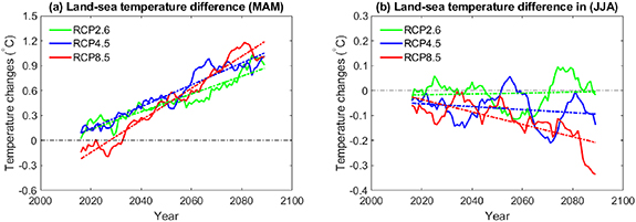
Figure 1. The land and sea temperature difference, the feedback run minus the no-feedback run, (t2m, °C) in (a) spring (MAM—March, April and May) and (b) summer (JJA—June, July and August) for RCP2.6, RCP4.5 and RCP8.5 scenarios. The temporal variations are based on a moving average of 10 years' data. The dash lines are the linear fits for temporal variations. The slopes of the linear fits in (a) are 0.106 °C decade−1, 0.132 °C decade−1, 0.193 °C decade−1 for RCP2.6, RCP4.5 and RCP8.5 scenarios respectively. The slopes of the linear fits in (b) are 0.002 °C decade−1, −0.006 °C decade−1, −0.025 °C decade−1 for RCP2.6, RCP4.5 and RCP8.5 scenarios respectively.
Download figure:
Standard image High-resolution imageThese temporal variations of land-temperature difference can be attributed to the changes in spatial patterns of near-surface air temperature (figure S2) and surface energy fluxes (figures S3 and S4) during spring and summer. The noticeable changes in near-surface air temperature due to BF in spring and summer are well observed across tundra areas of Siberia, northern Canada, Alaska and Scandinavian Mountains (figure S2). In general, BF-induced warming (e.g. most of them occurring in spring) or cooling effects (e.g. most of them occurring in summer) get reinforced in warmer RCPs, although the fraction of the BG-induced warming relative to the anthropogenic warming (i.e. (FB—NoFB)/(NoFB—hist)× 100) becomes smaller. Meanwhile, BF have increased upward (i.e. negative values) latent heat flux for both spring and summer in three RCPs (figure S3), these increased latent heat fluxes are mostly found in the areas where the vegetation changes from herbaceous species to woody species (figures S5(a)–(c)). In spring, the sensible heat flux is downward (e.g. positive values) in tundra areas and upward (i.e. negative values) in forest areas (figures S4(b), (f) and (j)). BF have reduced both upward and downward sensible heat flux (figures S4(a), (e) and (i)). In summer, the sensible heat flux is upward, and BF have decreased upward sensible heat flux or even turned them downward in the warmer RCPs (figures S4(k) and (l)). However, increased upward sensible fluxes due to BF are also found in tundra areas in Siberia for all RCPs (figures S4(c), (g) and (k)). Overall, the abovementioned changes in near-surface temperatures, and surface energy fluxes are associated with the major changes of the normalized physiognomy index (higher values indicate more woody species) and the normalized phenology index changes in three RCPs. For instance, the relative fraction of woody species increased in the taiga-tundra transition zones in the warmer scenarios, indicating that taller shrubs may encroach into the herbaceous tundra (figures S5(a)–(c)). Some deciduous forests (Larix) will be displaced by evergreen coniferous forests (e.g. Pinus) in Siberia (figures S5(d)–(f)).
3.2. Impacts of biogeophysical feedbacks on the atmospheric circulation in the Arctic
Figure 2 shows differences of MSLP between FB and NoFB runs for spring and summer during the last three decades for the different RCP scenarios. BF results in statistically significant circulation changes over the land in spring and over the Arctic Ocean in summer (figure 2). These changes become more evident in the RCP8.5 for both seasons. In spring, MSLP shows the largest reduction over the whole Arctic in the RCP8.5 scenario relative to the other two RCP scenarios (figure 2(e)). In summer, MSLP shows a significant increase over the Central Arctic, though this increase emerges already in the RCP4.5 scenario (figure 2(d)). Therefore, in summer the circulation over the Arctic Ocean becomes more anticyclonic/less cyclonic with the opposite occurring in spring in the 'FB' run. The circulation changes for the different atmospheric levels (850, 500 and 300 hPa) for the different RCP scenarios are shown in supplementary figures S6–S8. In spring, there is an increase of the geopotential height over the continents that become more prominent in the higher level. Under the RCP4.5 scenario, additionally, there is a decrease of the geopotential height over the Arctic Ocean. This decrease of the geopotential height over the ocean, coincident with an increase over the continents (dipole structure), is also observed in the RCP8.5 scenario. In summer, the same dipole structure is apparent in the RCP2.6 scenario. This dipole structure is also present under the RCP4.5 scenario, however, its position has changed. In contrast, under the RCP8.5 scenario, the geopotential height changes become positive over the whole Arctic Ocean. It should be noted that the geopotential height changes are partly insignificant, except in summer and under RCP8.5 in both seasons. Thus, we note that most pronounced and significant changes in the atmospheric circulation occur under the RCP8.5 scenario. Therefore, in the following section, we examine the factors that influence the baroclinic instability as triggers for cyclone genesis and growth with the focus on the RCP8.5 scenario results.
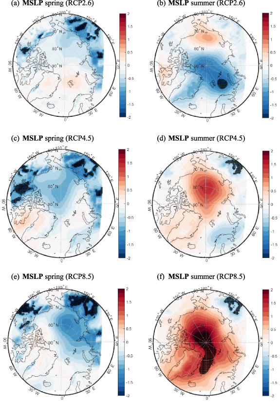
Figure 2. The effects of biogeophysical feedbacks on spring (a), (c), (e) and summer (b), (d), (f) mean sea level pressure (MSLP, hPa) averaged from 2070 to 2099 in the RCP2.6, RCP4.5 and RCP8.5 scenarios. Black dots indicate statistically significant differences (p < 0.05).
Download figure:
Standard image High-resolution image3.3. Changes in baroclinic instability
The primary factor for the generation and evolution of cyclones in northern high latitudes is the baroclinicity of the atmosphere. As outlined in section 2.4, a simple parameter measuring the baroclinic instability is the EGR, which depends on both the vertical static stability and the horizontal temperature gradients (through the thermal wind balance) in the atmosphere. Therefore, here we investigate the response of baroclinic instability to BF with focus on the RCP8.5 scenario. Spatial changes 'FB minus NoFB' for the other two RCP2.6 and RCP4.5 scenarios are presented in supplementary figures (figures S9 and S10).
In spring, the RCP8.5 warming scenario under no feedback conditions ('NoFB minus hist') leads to significant changes in EGR (figure 3(a)). EGR mostly increases over Alaska, Beaufort and Barents-Kara Seas, and decreases over the Eurasian continent, Norwegian Sea and over the Arctic Ocean. The static stability (Brunt–Vaisala frequency), which is a component of the EGR, decreases over most areas of the Arctic (figure 3(c)). Wind shear changes are in line with EGR changes (figure 3(e)). The BF ('FB minus NoFB') in spring increases EGR over parts of the Arctic Ocean (figure 3(b)). This is related with concurrent wind shear increase over the Norwegian and Laptev Seas, the Canadian Arctic and parts of the Eurasian continent (figure 3(f)). Further, the BF lead to a significant decrease of the static stability in the Arctic (figure 3(d)), i.e. the feedback triggers a further destabilization initiated by the warming scenario (figure 3(c)). These changes become more evident in the RCP8.5 scenario compared to the other two RCP4.5 and RCP2.6 scenarios (figures S9 and S10). However, the signal is not always statistically significant.
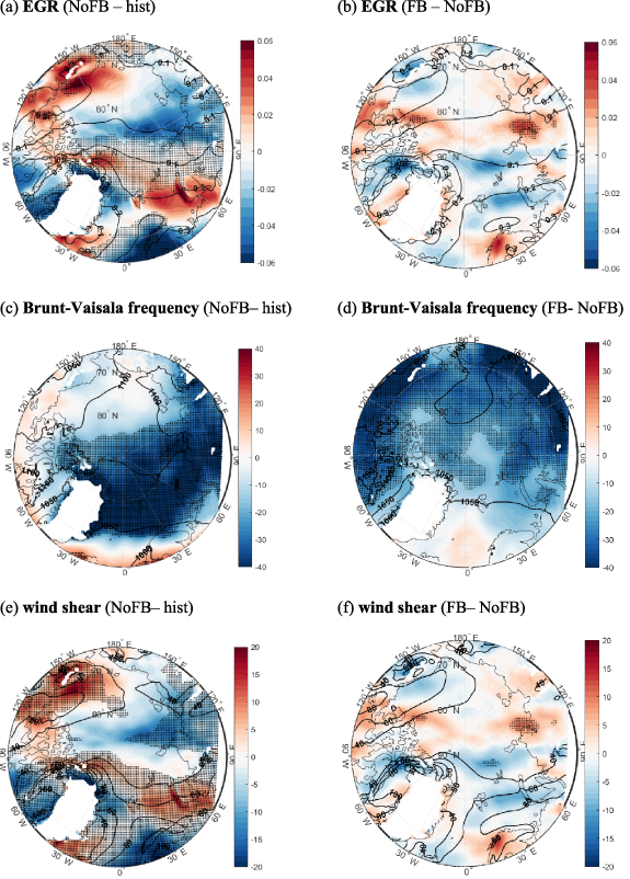
Figure 3. Changes of spring (March–May) Eady Growth rate, Brunt–Vaisala frequency and wind shear (1/day) between 1970–1999 and 2070–2099 periods in NoFB simulations (a), (c), (e), and between FB and NoFB simulations for 2070–2099 period (b), (d), (f) under RCP8.5 scenario. Black isolines show average EGR values for 1970–1999 (hist runs, (a), (c), (e)) and for 2070–2099 period (NoFB runs, (b), (d), (f)). Black dots indicate statistically significant differences (p < 0.05).
Download figure:
Standard image High-resolution imageIn summer, the RCP8.5 warming ('NoFB minus hist') effect on EGR (figure 4(a)) is similar strong as in spring. EGR increases over the Arctic Ocean as well as over the American continent (Alaska and Canadian Arctic). However, there are also negative significant changes seen over the Eurasian continent, Central Arctic and over the Barents-Kara Seas. In contrast to spring, the static stability increases everywhere in the Arctic in summer, with the smallest changes over the Barents-Kara seas (figure 4(c)). The wind shear increase follows as in spring, the pattern of the EGR change (figure 4(e)).
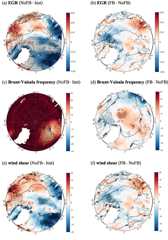
Figure 4. Same as in figure 3, but for summer (June–August).
Download figure:
Standard image High-resolution imageThe BF in summer ('FB minus NoFB') lead to an increase of EGR over Siberia and a strong decrease over the Canadian archipelago (figure 4(b)). The static stability is due to the feedbacks further increased over large areas of the Arctic Ocean, but is decreased over Siberia (figure 4(d)). The wind shear changes (figure 4(f)) again follow the regional changes in EGR.
The results show that BF noticeably modify the baroclinicity of the atmosphere in the warmer climate. Consequently, we may expect significant changes in cyclone characteristics in the Arctic in spring and summer due to BF.
3.4. Impacts of biogeophysical feedbacks on cyclone characteristics
Comparing the NoFB to hist runs, the cyclone frequency in the Arctic (>65° N) as a whole increases in both seasons with the greatest and significant changes in summer over the Arctic Ocean in the RCP8.5 scenario (table 1). In spring, the cyclone mean depth and size decrease in the Arctic including the Arctic Ocean. In summer, cyclone depth and size increase in the Arctic. Cyclone depth increase reaches its maximum over the Arctic Ocean in RCP8.5. Comparing the FB to NoFB runs, the cyclone frequency in the Arctic increases in spring and decreases in summer (table 2). Cyclone frequency increases six-fold in the Arctic in the RCP8.5 scenario relative to RCP2.6 in spring. In summer, a decrease in cyclone frequency is observed in RCP8.5. Cyclone mean depth decreases in FB in both seasons. While cyclone mean size decreases in RCP8.5, it increases under RCP2.6, for both spring and summer. Averaged over the Arctic Ocean (>75° N), BF increase the cyclone frequency with the greatest change in the RCP8.5 scenario in spring. In spring, cyclone frequency differences vary from +1% (RCP2.6) to +10% (RCP8.5). Impacts of BF on temporal variations of the cyclone characteristics for the Arctic Ocean (>75° N) and Arctic (>65° N) for different RCP scenarios in spring and summer are shown in supplementary figure S11. Impact of BF on cyclone characteristics are evident, and the impact varies depending on RCP scenario. The Arctic wide changes (tables 1 and 2) are aggregated from the regionally different changes in cyclone characteristics, and thus may not be representative for individual subregions. Therefore, it is important to highlight the regional pattern of cyclone changes.
Table 1. Changes (%/30 years) in cyclone frequency, depth and size for 'NoFB minus hist' by the end of the 21st century (2070–2099) for spring and summer from RCA-GUESS simulations under different RCP scenarios. Red (blue) values show increase (decrease). Bold and italics values indicate a statistical significance at p < 0.05. Values in thin light style indicate their statistically insignificance.
| Frequency (%) | Mean depth (%) | Mean size (%) | |||||
|---|---|---|---|---|---|---|---|
| Arctic | |||||||
| (>65° N) | Scenarios | Spring | Summer | Spring | Summer | Spring | Summer |
| NoFB—hist | RCP2.6 RCP4.5 RCP8.5 | 3.8 3.9 3.5 | 1.7 2.0 7.9 | −5.5 –5.5 −2.8 | 3.1 7.6 9.0 | −2.5 –1.9 1.1 | 0.9 2.2 2.2 |
| Arctic Ocean (>75° N) | Scenarios | Spring | Summer | Spring | Summer | Spring | Summer |
| NoFB—hist | RCP2.6 RCP4.5 RCP8.5 | 2.5 –0.2 5.2 | 7.6 14.8 23.8 | −7.9 –4.4 −3.3 | 5.0 13.9 17.7 | −4.4 –2.6 –0.6 | 0.2 1.9 1.6 |
Table 2. Changes (%/30 years) in cyclone frequency, depth and size for 'FB minus NoFB' by the end of the 21st century (2070–2099) for spring and summer from RCA-GUESS simulations under different RCP scenarios. Red (blue) values show increase (decrease). Bold values indicate a statistical significance at p < 0.05. Values in thin light style indicate their statistically insignificance.
| Frequency (%) | Mean depth (%) | Mean size (%) | |||||
|---|---|---|---|---|---|---|---|
| Arctic (>65° N) | Scenarios | Spring | Summer | Spring | Summer | Spring | Summer |
| FB—NoFB | RCP2.6 RCP4.5 RCP8.5 | 0.3 2.1 1.9 | 1.4 –1.1 −3.1 | −2.1 –2.2 −3.4 | −0.1 –1.1 −2.6 | 0.7 –0.1 −1.3 | 0.8 0.1 –0.2 |
| Arctic Ocean (>75° N) | Scenarios | Spring | Summer | Spring | Summer | Spring | Summer |
| FB—NoFB | RCP2.6 RCP4.5 RCP8.5 | 0.9 8.4 9.8 | 8.0 –3.7 −2.2 | 3.4 –0.8 −1.7 | −0.3 –1.8 −3.5 | 2.6 −0.1 −1.9 | 0.2 –0.4 −2.1 |
The spatial differences in the cyclone characteristics for 'NoFB minus hist' and 'FB minus NoFB' under RCP8.5 scenario for spring and summer are shown in figures 5 and 6. The figures show that the regional changes due to BF can be of a similar order as those due to the warming scenario, but the regional patterns are different. Under no feedbacks, the RCP8.5 leads in spring to a cyclone frequency increase over large areas in the Arctic. A decrease of cyclones is found over Barents-Kara Seas, in some parts of Canadian archipelago and western Siberia (figure 5(a)). Cyclone mean depth and size increase over the Beaufort and Chukchi Seas and eastern Siberia (figures 5(c) and (e)). BF lead to increase in the cyclone frequency over large parts of the Arctic Ocean and over Alaska and Yakutia, which become stronger in the RCP8.5 scenario (figure 5(b)), compared to RCP4.5 and RCP2.6 (figures S13(a) and S14(a)). A small decrease of cyclone frequency is seen over the Kara Sea and Canadian archipelago in all three RCP scenarios and additionally over the Norwegian Sea and eastern Yakutia (figure 5(b)). For cyclone mean depth and size, the BF can also lead to changes of comparable magnitude as the warming scenario, but with a counteracting effect in a few regions (figure 5). This is most prominent in the Beaufort and Chukchi Seas, where the RCP8.5 lead to an increased cyclone depth and size, but the BF work against it.
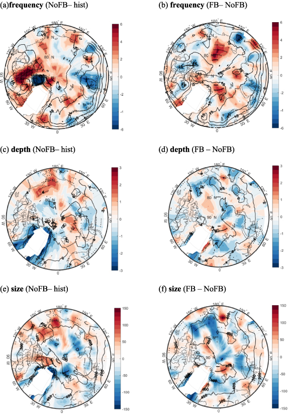
Figure 5. Changes of spring cyclone frequency (per season), depth (hPa) and size (km) between 1970–1999 and 2070–2099 periods in NoFB simulations (a), (c), (e), and between FB and NoFB simulations for 2070–2099 period (b), (d), (f) under RCP 8.5. Black isolines show average cyclone frequency values for 1970–1999 (hist runs, (a), (c), (e)) and for 2070–2099 period (NoFB runs, (b), (d), (f)). Black dots indicate statistically significant differences (p < 0.05).
Download figure:
Standard image High-resolution image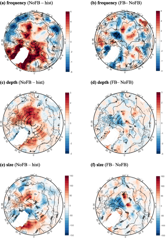
Figure 6. Same as in figure 5, but for summer (June–August).
Download figure:
Standard image High-resolution image
In summer, the cyclones increase over large parts of the Arctic Ocean in NoFB compared to hist runs under the RCP8.5 scenario (figure 6(a)), with stronger increase compared to spring. A decrease of cyclone frequency is observed over the continents. Similar patterns are seen for cyclone mean depth and size changes (figures 6(c) and (e)).
Spatial behavior of cyclone characteristics changes is quite patchy in the FB run in all three RCP scenarios (figures 6(b), S13 and S14). However, the overall cyclone frequency decreases in the Arctic including the Arctic Ocean in the RCP8.5 scenario (as shown in table 2). Like in spring, the changes in cyclone frequency, depth and size due to BF can be of similar order as those by the RCP8.5 warming scenario for specific regions with potential counteracting effects. The increased cyclone frequency, depth and size in the western Arctic Ocean due to RCP8.5 is reduced due to BF. In general, the spatial changes in cyclone size due to BF are in line with the changes of cyclone mean depth, i.e. reduced cyclone depth is accompanied with reduced cyclone size and increased depth goes hand in hand with increased size in summer.
There is a significant correlation between changes in cyclone characteristics and changes in land-sea thermal contrast induced by BF (figure S12). Importantly, its spatial patterns agree with those of changes in cyclone characteristics 'FB minus NoFB' particularly in spring (figure 5). This confirms that the mechanism through which the changes in cyclone characteristics are triggered by BF are associated with the changed land-sea thermal contrast. The latter is related to changes of baroclinic instability (EGR). The results show that changes in cyclone characteristics triggered by BF in both seasons are in line with changes in EGR over some areas but not all. In case of cyclone frequency, increase of EGR may lead to increased cyclone frequency, which is seen in parts over the Arctic Ocean in spring and summer and over continental regions in summer. As noted in Day and Hodges (2018b), increase of sea-land thermal contrast may lead also to increase of cyclone intensity (i.e. cyclone depth). Accordingly, over some areas the cyclone mean depth changes are in line with changes in EGR (and wind shear) in RCP8.5 (figures 3–6), such as over the Laptev Sea and north of the Canadian archipelago in spring and over the central Arctic Ocean and Laptev Sea in summer.
4. Summary and discussions
We have investigated the role of BF in changes of spring and summer cyclone activity in the Arctic to the end of the 21st century using a regional Earth system model (RCA-GUESS) with interactive dynamic vegetation under three RCP scenarios (from RCP2.6 to RCP8.5). We find that BF-induced changes in near-surface warming and surface heat fluxes lead to changes in land-sea temperature contrast and atmospheric stability. This, in turn, noticeably changes the atmospheric baroclinicity and, thus, leads to a change of cyclone activity in the Arctic. Our findings suggest that consideration of the BF in models can be important for correct simulations of the atmospheric circulation.
For the Arctic as a whole, our simulations suggest that the BF increase cyclone frequency in spring and increase/decrease the frequency in summer under different RCP scenarios. The maximum changes occur over the Arctic Ocean, with ca. +10% for spring under RCP8.5 and ca. −4% for summer under RCP4.5. For cyclone mean size and depth, these changes are smaller for both seasons. This indicates that biogeophysical processes play an important role in shaping the responses to anthropogenic forcing.
It would be interesting to assess BF effects on sea-ice and ocean conditions in the Arctic in spring-summer seasons and how this in turn affects and is affected by, cyclone activity. However, for this task, it would be necessary to additionally couple a sea-ice-ocean system within the architecture of a model like RCA-GUESS. We plan to do this in an upcoming study.
It should be noted that results obtained from regional climate models (RCMs) may be influenced by both lateral boundary conditions and RCM physics/parametrization which differ from model to model. As was noted in previous studies (e.g. Beniston et al 2007, Christensen and Christensen 2007), the large-scale forcing via the lateral boundary conditions from the driving GCMs can dominate simulations in winter, whereas in summer, when the circulation is weaker, the role of the RCM physics becomes more prominent. Akperov et al (2019) using an ensemble of different RCMs with various lateral boundary conditions and parametrizations showed that most models show similar behaviors in cyclone activity for most regions in the 21st century, including RCA-GUESS. In spite of this, it is important in further analysis of change in Arctic cyclone activity to include ensemble simulations with multiple RCMs, allowing internal and forced signals involved in changing cyclone activity to be distinguished.
Acknowledgments
This study was supported by the grants from Swedish Research Council FORMAS 2016-01201 and Swedish National Space Agency 209/19. We thank the National Supercomputer Center Bi cluster and the Rossby Center in SMHI (Swedish Meteorological and Hydrological Institute) for archiving the RCA-GUESS model code and data sets. This study is a contribution to the strategic research areas Modeling the Regional and Global Earth System (MERGE) and Biodiversity and Ecosystem Services in a Changing Climate (BECC) at Lund University. A R acknowledges the funding by the Deutsche Forschungsgemeinschaft (DFG, German Research Foundation)—Project number 268020496—TRR 172, within the Transregional Collaborative Research Center 'ArctiC Amplification: Climate Relevant Atmospheric and SurfaCe Processes, and Feedback Mechanisms (AC)3'. H M and A R were supported by the European Commission's Horizon 2020 project CHARTER (No. 869471). I I M acknowledges the support by the project funded by the Russian Science Foundation (RSF No. 19-17-00240). V A Semenov acknowledges the support by the project funded by the Russian Science Foundation (RSF No. 19-17-00242). M A acknowledges the support by the project funded by RFBR according to the research projects (Nos. 18-05-60216, 18-05-60111, 20-55-14003).
Data availability statement
The data that support the findings of this study are available upon reasonable request from the authors.