the Creative Commons Attribution 4.0 License.
the Creative Commons Attribution 4.0 License.
 | 24 Apr 2023
Atmospheric distribution of HCN from satellite observations and 3-D model simulations
Jeremy J. Harrison
Martyn P. Chipperfield
David P. Moore
Richard J. Pope
Christopher Wilson
Emmanuel Mahieu
Justus Notholt
Hydrogen cyanide (HCN) is an important tracer of biomass burning, but there are significant uncertainties in its atmospheric budget, especially its photochemical and ocean sinks. Here we use a tracer version of the TOMCAT global 3-D chemical transport model to investigate the physical and chemical processes driving the abundance of HCN in the troposphere and stratosphere over the period 2004–2016. The modelled HCN distribution is compared with version 4.1 of the Atmospheric Chemistry Experiment Fourier transform spectrometer (ACE-FTS) HCN satellite data, which provide profiles up to around 42 km, and with ground-based column measurements from the Network for the Detection of Atmospheric Composition Change (NDACC). The long-term ACE-FTS measurements reveal the strong enhancements in upper-tropospheric HCN due to large wildfire events in Indonesia in 2006 and 2015. Our 3-D model simulations confirm previous lower-altitude balloon comparisons that the currently recommended NASA Jet Propulsion Laboratory (JPL) reaction rate coefficient of HCN with OH greatly overestimates the HCN loss. The use of the rate coefficient proposed by Kleinböhl et al. (2006) in combination with the HCN oxidation by O(1D) gives good agreement between ACE-FTS observations and the model. Furthermore, the model photochemical loss terms show that the reduction in the HCN mixing ratio with height in the middle stratosphere is mainly driven by the O(1D) sink with only a small contribution from a reaction with OH. From comparisons of the model tracers with ground-based HCN observations we test the magnitude of the ocean sink in two different published schemes (Li et al., 2000, 2003). We find that in our 3-D model the two schemes produce HCN abundances which are very different to the NDACC observations but in different directions. A model HCN tracer using the Li et al. (2000) scheme overestimates the HCN concentration by almost a factor of 2, while a HCN tracer using the Li et al. (2003) scheme underestimates the observations by about one-third. To obtain good agreement between the model and observations, we need to scale the magnitudes of the global ocean sinks by factors of 0.25 and 2 for the schemes of Li et al. (2000) and Li et al. (2003), respectively. This work shows that the atmospheric photochemical sinks of HCN now appear well constrained but improvements are needed in parameterizing the major ocean uptake sink.
- Article
(1185 KB) -
Supplement
(1194 KB) - BibTeX
- EndNote


Hydrogen cyanide (HCN) is one of the most abundant cyanides in the atmosphere (Singh et al., 2003) and can influence the nitrogen cycle and reactive nitrogen (NOx) (Li et al., 2000, 2003, 2009). Previous modelling studies (Li et al., 2000, 2003, 2009; Singh et al., 2003; Kleinböhl et al., 2006) have shown that the HCN variability is mainly determined by biomass burning, as the dominant source, and by ocean uptake, as the major tropospheric sink. HCN is, in fact, released into the atmosphere predominantly by biomass burning events with only a minor contribution from industrial activities. In addition, Li et al. (2000, 2003) suggest that ocean uptake is the major loss process at the surface with a non-negligible contribution from the oxidation by OH radicals in the troposphere (Cicerone and Zellner, 1983). As a result, the HCN tropospheric lifetime is estimated at about 5 months (Singh et al., 2003; Li et al., 2000, 2003). The stratospheric HCN reduction instead is caused by photochemical loss, with a resulting 4–5-year lifetime in the stratosphere (Cicerone and Zellner, 1983; Li et al., 2000, 2003). Due to its low chemical reactivity and long lifetime, HCN is a good atmospheric tracer of biomass burning events. However, the atmospheric HCN budget and the processes driving its variability are still not fully understood (Li et al., 2003; Singh et al., 2003). The rate constant for the reaction between HCN and OH and the rate at which HCN is reduced by ocean uptake still have a number of significant uncertainties. The present study aims to clarify some of the key uncertain aspects in HCN sources and sinks using 3-D model simulations, satellite solar occultation data, and ground-based measurements of HCN in the atmosphere.
HCN column measurements from ground-based Fourier transform infrared (FTIR) spectrometers are available at several sites from the Network for the Detection of Atmospheric Composition Change (NDACC) (De Mazière et al., 2018). These measurements are an important source of information on the spatial and temporal distribution of HCN but are too sparse to represent a strong global constraint on HCN emissions and removal processes. HCN volume mixing ratio (VMR) profiles measured during balloon-borne campaigns provide more accurate information on the vertical distribution of HCN (Kleinböhl et al., 2006) but with limitations in spatial and temporal coverage. Some limitations of the balloon observations are overcome by satellite observations which offer global coverage and can place the balloon profiles measured at a few locations into a wider context, also extending the sensing range to the stratosphere. Together, this information provides a good constraint on the HCN concentrations and processes driving HCN variability on a global scale.
The Atmospheric Chemistry Experiment Fourier transform spectrometer (ACE-FTS), launched in 2004, was one of the first satellite instruments to measure HCN VMRs in the lower stratosphere. ACE-FTS measures HCN VMRs from the middle troposphere up to ∼ 42 km with ∼ 3 km vertical resolution (Boone et al., 2005, 2020; Sheese et al., 2017); the extended altitude range allows us to test the HCN stratospheric loss, not otherwise possible with balloon-borne missions. The Microwave Limb Sounder (MLS) on the Aura satellite has also been measuring HCN mixing ratios since its launch in 2004. Both satellites have been used, frequently in combination, to study HCN variability in the upper troposphere and lower stratosphere (UTLS) and the biomass burning emission impact on the HCN concentrations (Pumphrey et al., 2006, 2018; Li et al., 2009; Sheese et al., 2017; Park et al., 2021). The MLS v5.0 data product for HCN has extremely large systematic errors in the lower stratosphere. For this reason, the data are not recommended for scientific use outside the upper stratosphere at pressures greater than 21 hPa (altitudes below ∼ 27 km) (Livesey et al., 2022), so we decided to perform our study using only ACE-FTS data.
Atmospheric chemical transport models (CTMs) are excellent tools for testing our understanding of atmospheric processes using a variety of observations and for deriving global tracer budgets. Here we use a tracer version of the detailed TOMCAT 3-D CTM adapted to include the processes driving HCN variability (Bruno et al., 2022a). TOMCAT is used in order to quantify the role played by the different stratospheric HCN loss mechanisms in determining the HCN variability observed from satellite measurements and to assess how well currently available parameterizations perform in simulating HCN. Two rate coefficients for HCN oxidation by OH radicals have been compared, one based on the current JPL recommendation, which was last revised in 1983 (Burkholder et al., 2015, 2019), and the other from Kleinböhl et al. (2006) and Strekowski (2001). We show that the JPL-recommended rate largely overestimates the HCN loss, while the use of the other Kleinböhl et al. (2006) rate coefficient significantly improves the agreement between the measurements and the model. ACE-FTS version 4.1 HCN data (Bernath et al., 2021) have been used to validate the modelled HCN distribution over the years 2004–2016. The model tracers have also been used to understand the ocean uptake contribution in tropospheric HCN variability. Two ocean uptake fluxes from Li et al. (2000) and Li et al. (2003) were added into the TOMCAT model and evaluated using ground-based FTIR HCN measurements from the NDACC network.
2.1 Satellite observations
The Atmospheric Chemistry Experiment Fourier transform spectrometer (ACE-FTS) is a high-spectral-resolution (0.02 cm−1) limb sounder instrument on board the Canadian Science Satellite mission (SCISAT). SCISAT moves along a circular low Earth orbit at an altitude of 650 km with an inclination of 74∘ and an orbit period of 97.7 min (Bernath et al., 2005). This orbit gives a sampling pattern with a high density of observations at high latitudes. The original aim of the SCISAT mission was to obtain complete insight into the physical and chemical processes driving the distribution of ozone by measuring changes in atmospheric composition, in particular in polar regions. ACE-FTS operates in the infrared absorption spectrum over the range 750–4400 cm−1 (2.2 to 13.3 µm) using the solar occultation technique, measuring a wide range of molecules in the upper troposphere and stratosphere (Bernath et al., 2005). Its profiles have been widely used as a reference for interpreting ground-based and nadir satellite measurements of HCN and to help in validating tropospheric–stratospheric transport in atmospheric models (Park et al., 2013; Viatte et al., 2014; Glatthor et al., 2015; Sheese et al., 2017). The retrieved HCN profiles extend from the middle troposphere (∼ 6–8 km) to ∼ 42 km with a vertical resolution on the order of ∼ 3 km (Boone et al., 2005, 2020). ACE-FTS observations extend higher than the profiles measured by balloon-borne missions (Kleinböhl et al., 2006), allowing us to investigate stratospheric HCN variability and to test the different processes driving HCN loss. Here we present ACE-FTS version 4.1 HCN data (Bernath et al., 2021), the most recent update version, and use it to evaluate different modelled HCN tracers.
Figure 1 shows the seasonal ACE-FTS of the sample year 2008–2009 HCN zonal mean cross sections in 10∘ latitude bins. To highlight the HCN stratospheric distribution, the dashed black line shows the seasonal average location of the tropopause, based on the World Meteorological Organization (WMO) thermal tropopause definition (Maddox and Mullendore, 2018) using ECMWF ERA-Interim reanalyses (Dee et al., 2011). The first panel of Fig. 1 shows the December–February (DJF) season, which exhibits a high upper-tropospheric HCN concentration in the Southern Hemisphere (SH) from midlatitudes to high latitudes. In the March–May (MAM) season an enhancement of upper tropospheric HCN is observed in the Northern Hemisphere (NH) from the tropics to midlatitudes, while in the June–August (JJA) season the enhancement is observed in the NH midlatitudes to high latitudes. The observed behaviour is attributable to biomass burning emissions during the wildfire seasons in the tropical and midlatitude regions, respectively. During the September–November (SON) season an enhancement of HCN in the upper troposphere is observed over southern tropics, due to biomass burning emissions from South America, Africa, and South-East Asia.
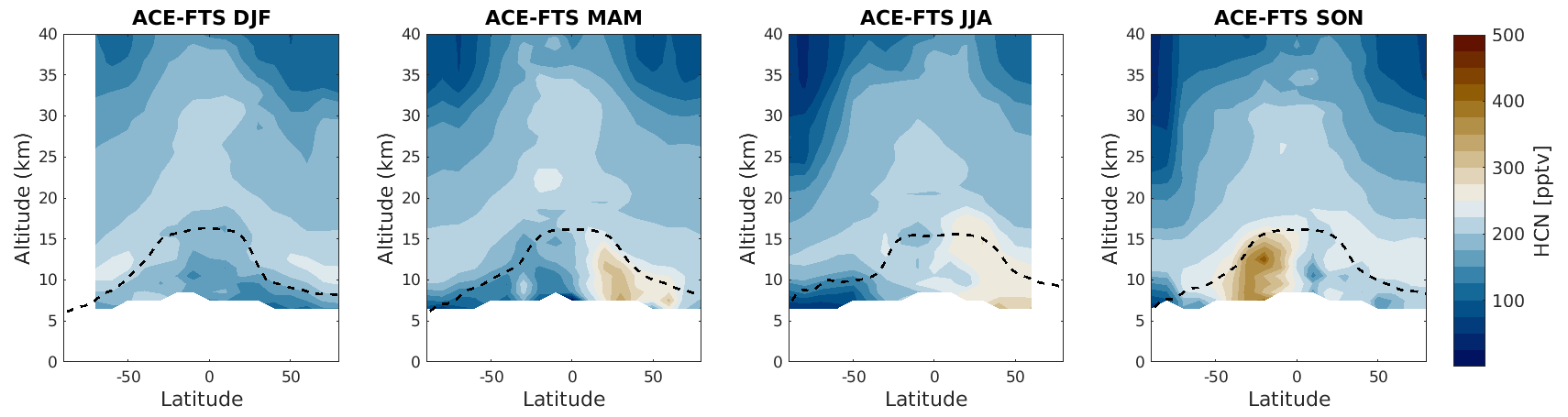
Figure 1Latitude–height cross sections of ACE-FTS HCN zonal mean profiles (pptv) in 10∘ latitude bins for four seasons, December–February (DJF), March–May (MAM), June–August (JJA), and September–November (SON), from December 2008 to November 2009. The dashed black lines show the season-averaged location of the thermal tropopause (Maddox and Mullendore, 2018) based on ECMWF ERA-Interim reanalyses for the same periods.
Figure 2 shows the time–altitude cross sections of the 2-month mean HCN mixing ratios measured by ACE-FTS averaged over three 30∘ latitude bands. Here, the strong HCN tropospheric seasonal variability is clearly visible and is followed by a similar seasonal cycle in the stratosphere at all latitudes, in agreement with Park et al. (2021). During the months following the period of high tropospheric HCN concentration, a large amount of HCN is transported to the stratosphere, where it persists for the following years. In particular, after the El Niño events, which influence the fire season of South-East Asia, this amount is notably high. Looking specifically at the tropical region, two of the largest El Niño events ever recorded in Indonesia, in 2006 and 2015, are highlighted by an extremely high concentration of HCN emitted during peat fires. During the months following the two events, a large quantity of HCN was transported to the stratosphere and persisted for a longer time than the typical seasonal variation. Specifically, after the 2015 Indonesian fire season, the HCN transported to the stratosphere persisted for the following 2 years before being completely reduced. Sheese et al. (2017) observed the transport of the HCN from the upper troposphere to the lower stratosphere during January and February 2016 and its persistence during the entire year using ACE-FTS measurements. This behaviour is also visible in the latitude band 15–45∘ S.
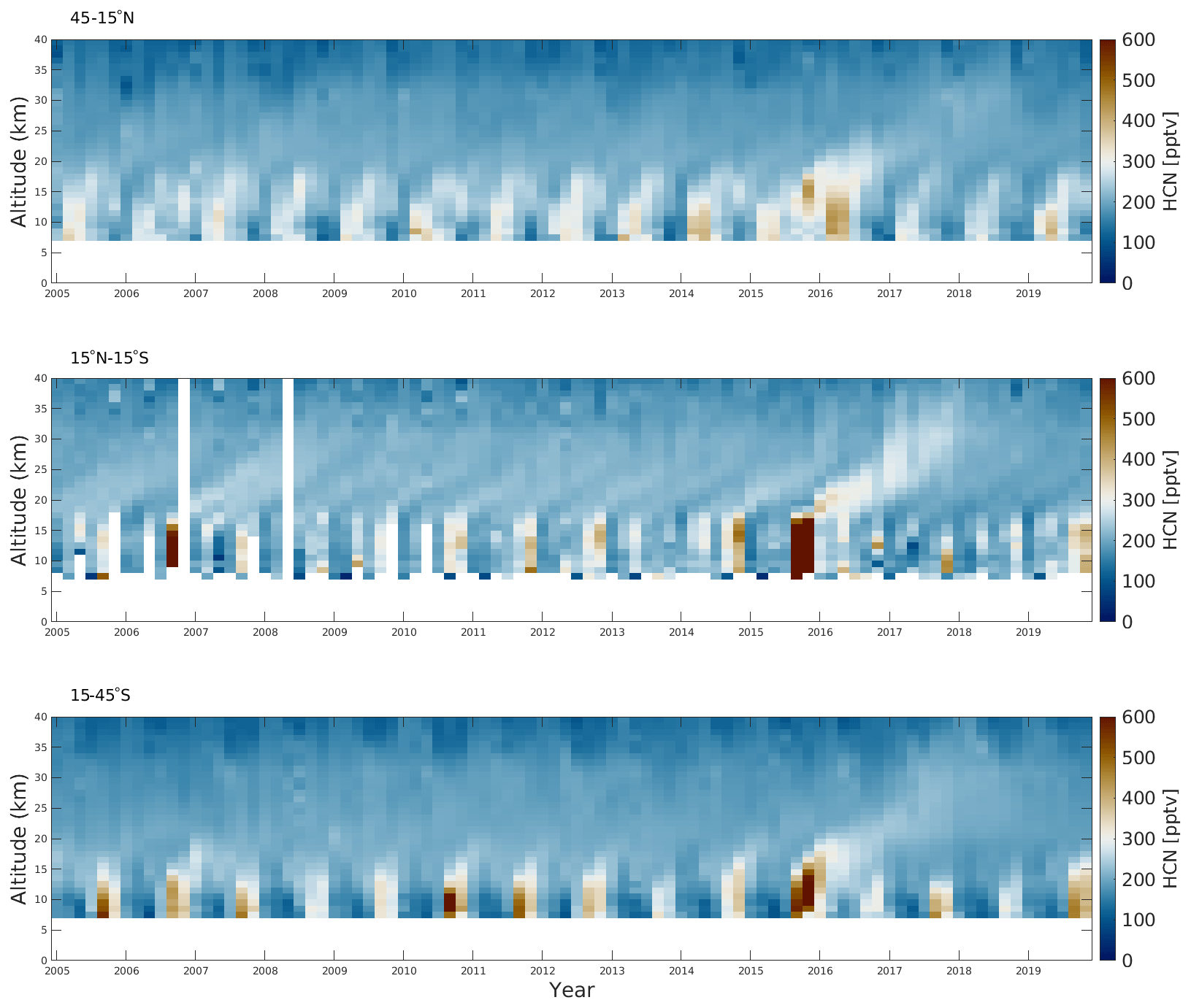
Figure 2Time–altitude sections of 2-month mean HCN mixing ratios (pptv) from ACE-FTS averaged into three 30∘ latitude bins, 45–15∘ N, 15∘ N–15∘ S, and 15–45∘ S, for 2005–2020. Note that the colour scale saturates and the maximum observed HCN mixing ratio in the tropical band in 2015 is over 1300 pptv.
2.2 Ground-based FTIR observations
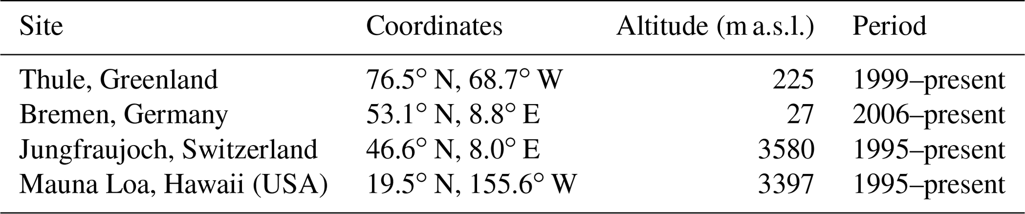
NDACC is an international global network of more than 90 ground-based stations that measure atmospheric composition in order to detect long-term changes and trends in the chemical and physical state of the atmosphere (De Mazière et al., 2018). The stations employ a variety of techniques and instruments, and observations at some sites extend from the early 1990s. Because of the different instruments and station set-ups, not all species are available at all stations. The Fourier transform infrared (FTIR) instruments are used at around 25 NDACC sites. They consist of a high-quality FTIR spectrometer combined with a high-precision solar tracker, which records the direct solar absorption spectra in the mid-infrared spectral region. The instruments work only under clear-sky conditions; i.e. the instrument view must be free of clouds, and no measurements are possible during the night, including, of course, polar night. This impacts the ground-based FTIR sampling frequency, with typically an average of 120 observation days every year, when considering all sites. Note, however, that for some stations, yearly coverage can be significantly larger, lying regularly in the range 240–270 d of measurements every year. The NDACC sites which measure HCN vertical columns are distributed globally, with a higher concentration in the NH, especially in Europe and North America. Here we selected HCN ground-based measurements from four sites (Table 1), having a long and continuative measurements time series: Thule (Greenland) at NH high latitudes, Bremen (Germany) and Jungfraujoch (Switzerland) at NH midlatitudes, and Mauna Loa (Hawaii, USA) in the tropics.
Table 1Ground-based NDACC FTIR observation sites used in this study.
We investigate HCN variability using an updated version of the TOMCAT 3-D chemical transport model (CTM). TOMCAT is an Eulerian offline 3-D global CTM used for a wide range of tropospheric and stratospheric chemistry studies. It was originally developed by Chipperfield et al. (1993) as two different models used for tropospheric and stratospheric studies, respectively, called TOMCAT and SLIMCAT. The two models were subsequently combined into the TOMCAT–SLIMCAT unified model (Chipperfield, 2006; Monks et al., 2017), which hereafter we call TOMCAT. TOMCAT has been used in a large number of studies and performs well in simulations of tropospheric (e.g. Pope et al., 2020) and stratospheric (e.g. Chipperfield et al., 2018) chemistry.
TOMCAT typically uses a flexible horizontal and vertical resolution with a σ−p vertical coordinate system. The vertical grid includes the surface σ, level which follows the terrain and pure pressure levels at higher altitudes up to 10 Pa (about 60 km). In the present study, the model was run at a spatial resolution of on a 60-level altitude grid from 2000 to 2016. The meteorology of the model is forced by humidity, temperature, and winds from ERA-Interim reanalyses provided by the European Centre for Medium-Range Weather Forecasts (ECMWF) with a 6 h time resolution (Berrisford et al., 2011; Dee et al., 2011). The meteorological information is linearly interpolated to fit with the time step and the spatial grid chosen for the model run. Natural and anthropogenic surface emissions are included in the model on a resolution and re-gridded onto the model spatial grid. The HCN emissions are extracted from some principal emission datasets: the Coupled Model Intercomparison Project Phase 6 (CMIP6) for anthropogenic and ocean emissions (Eyring et al., 2016), the Chemistry-Climate Model Initiative (CCMI) for a fixed annual biogenic emission dataset (Morgenstern et al., 2017), and Global Fire Emissions Database Version 4 (GFED4) for the biomass burning emissions (Randerson et al., 2017).
3.1 Upper-troposphere–stratosphere HCN loss
The TOMCAT simulation included four idealized HCN tracers (HCN1 to HCN4) to test the different atmospheric loss mechanisms of HCN. For each of these tracers, the global surface HCN volume mixing ratio (VMR) was constrained to a fixed value of 200 ppt, approximately the background tropospheric VMR measured during the Transport and Chemical Evolution over the Pacific (TRACE-P) aircraft campaign and modelled by Li et al. (2003) and Singh et al. (2003). The HCN atmospheric chemistry was modelled using the parameters summarized in Table 2. The main focus here is on the HCN removal process via oxidation by OH radicals and the comparison of the two different reaction rates, the recommended rate proposed by JPL (Burkholder et al., 2015, 2019) and the rate presented by Kleinböhl et al. (2006) based on the experimental measurements of Strekowski (2001). The other loss process included in the four tracers is the HCN reaction with O(1D) (Kleinböhl et al., 2006; Strekowski, 2001). The loss of HCN by photolysis is very slow and can be ignored (Burkholder et al., 2019).
Burkholder et al. (2015, 2019)Strekowski (2001); Kleinböhl et al. (2006)Strekowski (2001); Kleinböhl et al. (2006)Burkholder et al. (2019)Table 2HCN atmospheric photochemical loss mechanisms used for the different TOMCAT model tracers.
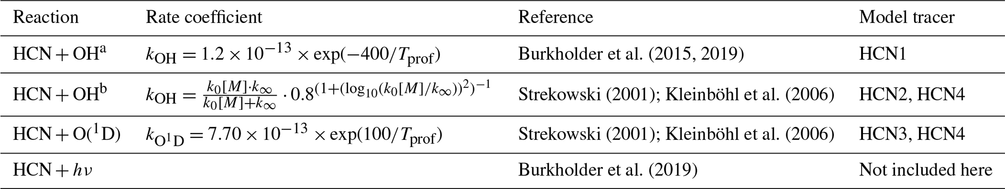
a The rate coefficient is expressed in cm3 molec.−1 s−1, and Tprof is the temperature profile expressed in kelvin (K). b k0 is given in cm6 molec.−2 s−1, k∞ is in cm3 molec.−1 s−1, and [M] is the molecular air density.
Figure 3 compares the four model tracers with example average profiles measured by ACE-FTS averaged over 60∘ latitude bands. Tracer HCN1 includes only the JPL-recommended rate for HCN oxidation by a reaction with OH. This tracer substantially underestimates the amount of HCN in the stratosphere. The HCN1 profile shows a drastic reduction in the HCN VMR at altitudes above ∼20 km, where the measured value is greater than 150 pptv. HCN2 is used to evaluate the HCN oxidation by OH radicals using the Kleinböhl et al. (2006) rate constant. For this tracer the model VMRs are closer to the measurements but, above 30 km at high latitudes in both hemispheres, the modelled HCN amount clearly overestimates the ACE observations by about 60 pptv. Introducing the HCN destruction by O(1D) this gap between observations and the model is greatly reduced. Considering the O(1D) sink alone (tracer HCN3) or in combination with the HCN reaction with OH (tracer HCN4), we obtain a much more reasonable agreement with the measured HCN profile in the middle–upper stratosphere. Tracers HCN3 and HCN4 show that the stratospheric HCN loss is driven by the reaction with O(1D). This good agreement is further support that loss of HCN by photolysis in the stratosphere is negligible.
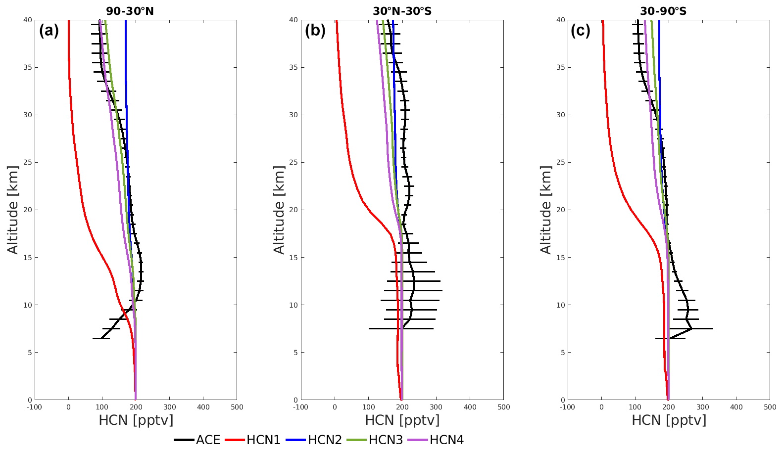
Figure 3Average HCN profiles for March–May 2009 for four TOMCAT model tracers (HCN1–HCN4) compared with the profiles measured by ACE-FTS with ±1 median absolute deviation for latitude bands 90–30∘ N (a), 30∘ N–30∘ S (b), and 30–90∘ S (c). See Table 2 for details of the photochemical loss reactions included in the different model HCN tracers.
3.2 Ocean uptake
Li et al. (2000) and Li et al. (2003) both modelled HCN variability and developed two different schemes to reproduce the ocean uptake (Li et al., 2000, 2003). The first scheme was developed to test, using the 3-D model GEOS-Chem (Goddard Earth Observing System chemistry model), the hypothesis that the biomass burning provides the main HCN source and the ocean uptake provides the main sink by focusing on the HCN seasonal features (Li et al., 2000). The Li et al. (2003) scheme was introduced into the GEOS-Chem model to perform new simulations with a longer HCN lifetime and weaker global sources than those of the previous study (Li et al., 2000), in order to match the TRACE-P constraints. The authors of Li et al. (2003) assert that their model achieved a similar or better simulation than in the study of Li et al. (2000).
In our study, a second set of six HCN tracers was implemented in TOMCAT to evaluate the two different ocean uptake schemes from Li et al. (2000) and Li et al. (2003). For these tracers the atmospheric photochemical loss was included as in tracer HCN4, with the HCN reactions with OH (using the rate constant from Kleinböhl et al., 2006) and O(1D), as this tracer gave the best model representation of stratospheric HCN variability compared to ACE-FTS.
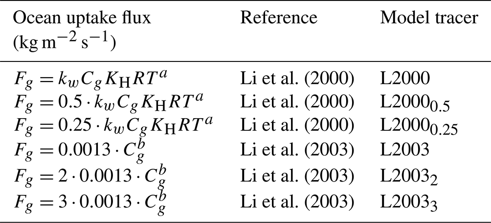
The ocean uptake flux of HCN proposed by Li et al. (2000) is defined as
where (m s−1) is the air-to-sea transfer velocity with u (m s−1), the wind speed at 10 m, and the dimensionless parameter is the Schmidt number of HCN in water, with ν (m2 s−1) as the kinematic viscosity and D (m2 s−1) as the diffusion coefficient of HCN in water. Cg (kg m−3) is the concentration of HCN in surface air, KH is the temperature-dependent Henry’s law constant defined as KH=12 M atm−1 at 298 K, and K. R=287.05 J kg−1 K−1 is the gas constant, and T (K) is the sea surface temperature.
The second ocean uptake scheme from Li et al. (2003) uses the results of a box model of the marine boundary layer (MBL) to derive an oceanic deposition velocity of 0.13 cm s−1 (Singh et al., 2003). The resulting flux is defined as
where Cg (kg m−3) is the HCN concentration near the surface.
The NDACC ground-based column measurements are used to evaluate the ocean uptake schemes, which act as the HCN surface sinks in the model, due to the large impact on the HCN budget and mean tropospheric VMR. The TOMCAT simulation is sampled at each NDACC station location, and the profiles are smoothed using the instrument-specific averaging kernels. The total column time series are then compared as shown in Figs. S1–S4 in the Supplement. The agreement is evaluated considering the values of the root mean square error (RMSE) and the coefficient of determination (R2) in reference to the measurements (Tables S1–S2 in the Supplement).
Li et al. (2000)Li et al. (2000)Li et al. (2000)Li et al. (2003)Li et al. (2003)Li et al. (2003)Table 3HCN ocean uptake rates used for the different TOMCAT model tracers.
Tracers L2000 and L2003, which make use of the two published schemes from Li et al. (2000) and Li et al. (2003), respectively, show a good agreement with NDACC total column time series only in terms of the HCN seasonality. In fact, L2000 and L2003 show the highest RMSE values among all the tracers and a strongly negative R2 at each location. The two tracers give greatly different results in our 3-D model compared to the HCN amount measured by FTIR instruments; L2000 underestimates the HCN total columns, with the values being almost two-thirds of the observed values, while L2003 greatly overestimates them, with the model being almost double the FTIR-measured values. The observed mismatch is attributable to the ocean uptake fluxes being unable to capture contributions of this process to the HCN variability. We therefore need to scale the two sinks, in different directions, in order to reach a better representation of HCN variability. The new tracers, L20000.5 and L20000.25, are created by applying the scaling factors 0.5 and 0.25, respectively, to reduce the Li et al. (2000) ocean uptake flux, while the tracers L20032 and Li20003 apply factors of 2 and 3, respectively, to the Li et al. (2003) flux in order to increase the HCN ocean uptake.
The tracers including the scaled ocean uptake schemes show a substantial improvement in the agreement with the NDACC measurements. In particular, the best agreement, considering the RMSE and R2 values, is obtained by reducing the HCN flux in the Li et al. (2000) scheme by three-quarters or by doubling the Li et al. (2003) flux in the L20032 tracer.
Figure 4 shows a comparison between the measured HCN total column time series and the two best-performing tracers, L20000.25 and L20032, characterized by the lowest RMSE and a large R2, and the worst one, L2003. HCN total columns from the L2003 model tracer are larger than the HCN measured by FTIR instruments at all the locations; it is clearly visible especially for Jungfraujoch, where the HCN estimated by L2003 is more than twice that the measured one. Both L20000.25 and L20032, the best-performing model tracers, agree very well with the measured values, confirming that both ocean uptake schemes published by Li et al. (2000, 2003) need to be scaled to be more accurate in reproducing HCN variability.
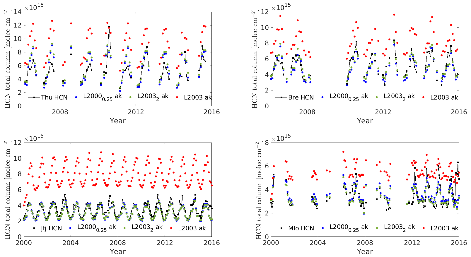
Figure 4HCN total column time series (molec. cm−2) measured at four NDACC stations (Thule (Thu), Bremen (Bre), Jungfraujoch (Jfj), and Mauna Loa (Mlo); black lines) and modelled by the L20000.25 (blue dots), L20032 (green dots), and L2003 (red dots) tracers (with averaging kernels applied; ak). Note the different time periods at the different stations.
3.3 Atmospheric lifetime and global budgets
The global budgets of atmospheric HCN for the model tracers L2000, L2003, and L20000.25 are shown in Table 4. Here we report only the two tracers using the original ocean uptake schemes from Li et al. (2000, 2003), which have the worst performance, and the best one using the ocean uptake from Li et al. (2000) scaled by 0.25. The total atmospheric burdens of HCN are 0.33, 0.89, and 0.55 Tg N, respectively, reflecting the HCN concentration underestimation of the L2000 tracer and the overestimation of the L2003 tracer, while the burden of L20000.25 is close to the values reported in Li et al. (2000, 2003) and Singh et al. (2003). Each HCN tracer uses the same emission scheme, with biomass burning as the main contribution, producing 2.42 Tg N yr−1. Ocean uptake provides the main sink for all the tracers, 2.36 Tg N yr−1 in L2000, 2.32 Tg N yr−1 in L2003, and 2.38 Tg N yr−1 in L20000.25, which all largely balance the emissions despite the variation in the first-order rate of uptake (i.e. the change in atmospheric HCN burden compensates). The sink from a reaction with OH is 0.05, 0.12, and 0.12 Tg N yr−1 for L2000, L2003, and L20000.25, respectively. Despite its importance for determining the stratosphere loss of HCN, the reaction with O(1D) is a relatively very small sink globally, 7 × 10⁻⁴ for the L2000 tracer, 1.9 × 10⁻³ for L2003, and 1.9 × 10⁻³ Tg N yr−1 for L20000.25. The resulting tropospheric lifetimes are 1.6, 4.4, and 2.6 months for the three tracers reported in Table 4.
The budgets of the L20000.25 tracer, which best reproduces the HCN variability, are in good agreement with the HCN budgets of Li et al. (2000), while the ocean uptake loss and the emissions are substantially larger than the Li et al. (2003) and the Singh et al. (2003) results. Li et al. (2003) estimate a global HCN loss to the ocean of 0.73 Tg N yr−1, and Singh et al. (2003) estimate one of 1.0 Tg N yr−1; both of these estimations are less than a half of the ocean uptake calculated in the present study. Similarly our emissions are more than twice the total emissions from Li et al. (2003), 0.63 Tg N yr−1 from biomass burning and 0.2 Tg N yr−1 from residential coal burning, and Singh et al. (2003), 1.1 Tg N yr−1. The resulting global mean atmospheric lifetime is also in agreement with the range of 2.1–4.4 months calculated by Li et al. (2000).
Table 4Global burden, budget terms, and atmospheric lifetimes for three model HCN tracers.
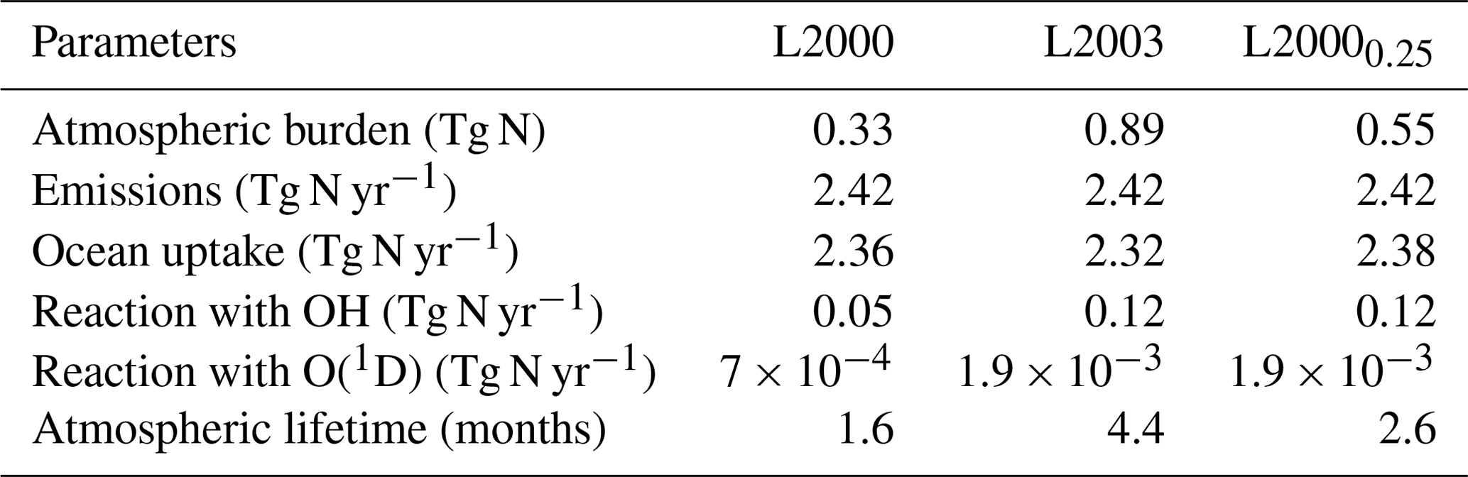
Figure 5 shows the simulated global mean distributions of HCN at the surface level for the six tracers created to test the ocean uptake schemes during September 2009. Higher surface concentrations of HCN (>1000 pptv) are observed over the biomass burning regions of South-East Asia, Central America, and Central Africa. The HCN surface concentrations are very low (<100 pptv) over the oceans, especially at high latitudes in the SH. This is due to the remote position from any HCN biomass burning emission sources, reflecting the role of the ocean uptake as the major removal mechanisms in the marine boundary layer. It is important to highlight that the lack of ground-based observations in the SH is a limitation for better constraining the HCN distribution in this part of the world.
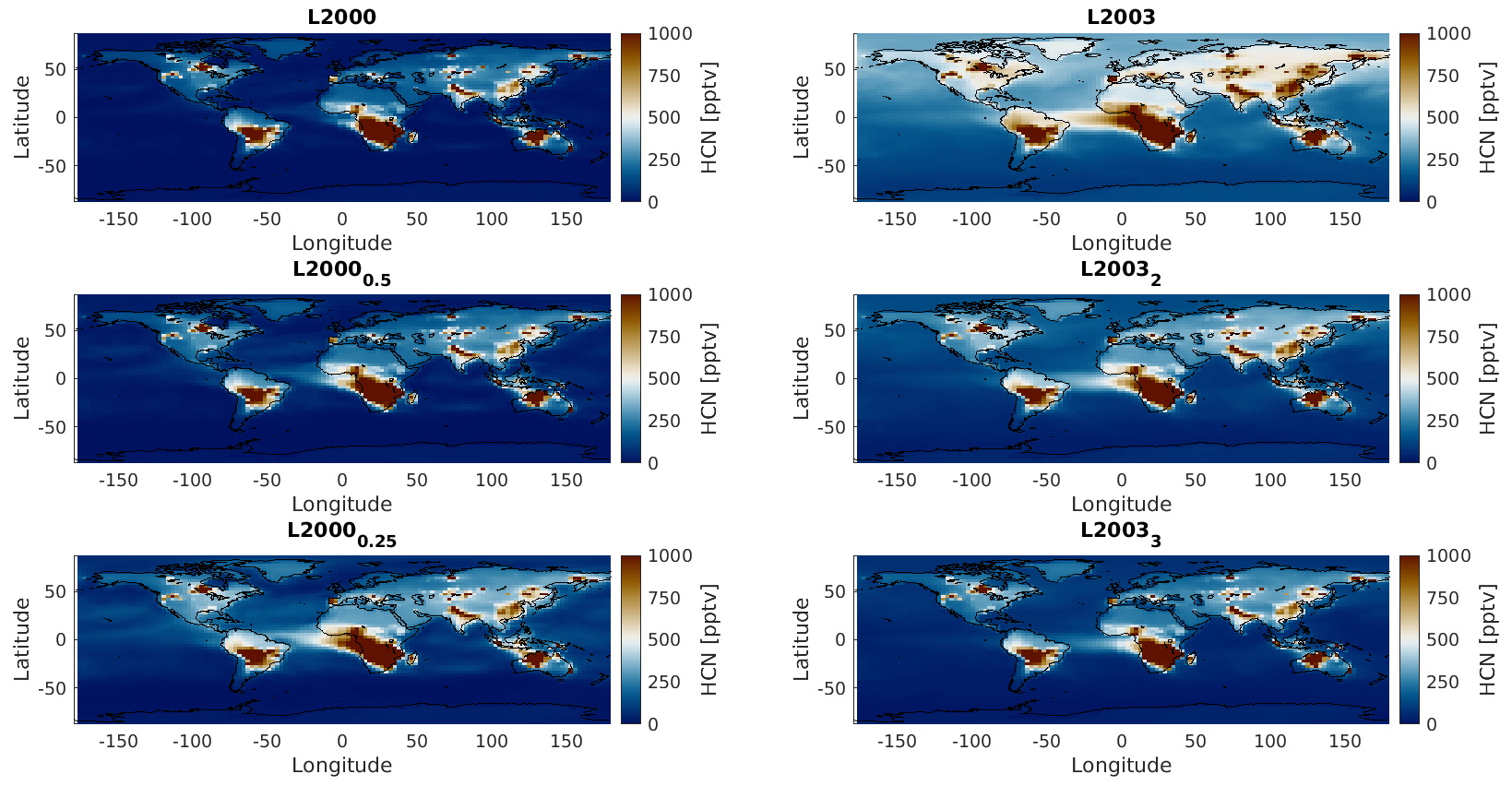
Figure 5Simulated global distributions of HCN (pptv) for six model tracers, L2000–L20033, at the surface level for September 2009.
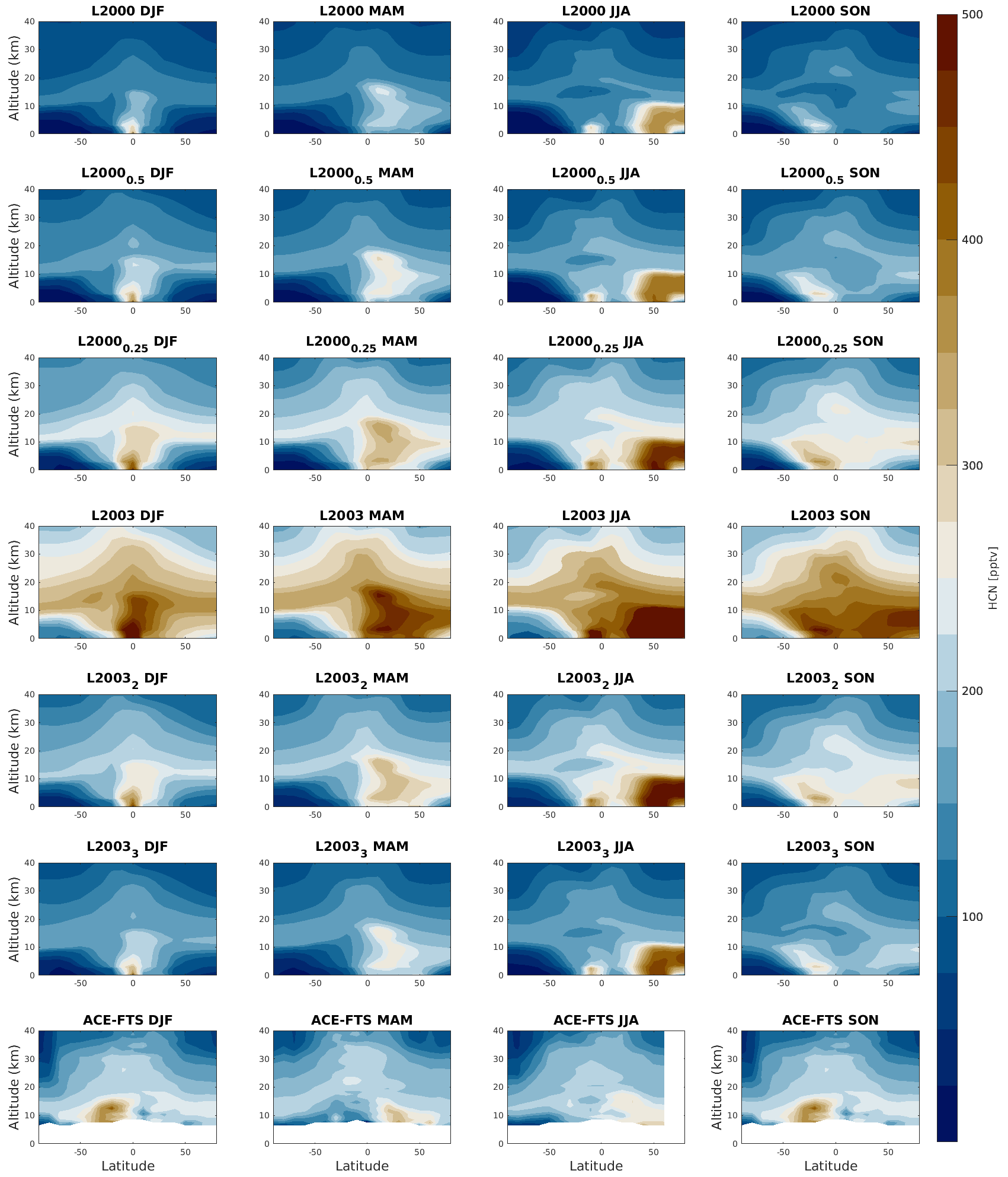
Figure 6Seasonal mean latitude–height zonal mean cross sections from December 2008 to November 2009 of HCN zonal means in 10∘ latitude bins for six TOMCAT HCN tracers and ACE-FTS measurements (on the rows).
Figure 6 shows the seasonal latitude–height zonal mean cross sections for December 2008–November 2009 for the model tracers used to test the Li et al. (2000) and Li et al. (2003) ocean uptake schemes. This figure reveals the presence of a generally asymmetric distribution of HCN between the two hemispheres, with a higher concentration of HCN in the NH, which has more biomass burning regions. As shown in Fig. 1 and reported in the last row of Fig. 6, HCN also has a strong seasonal pattern linked to the biomass burning emissions during the seasons of large wildfires. All the tracer cross sections generally reproduce this seasonal behaviour with some small differences. ACE-FTS data during season DJF exhibit a high HCN concentration in the upper troposphere over the SH between midlatitudes and high latitudes (Fig. 1). The model tracers highlight a band of high HCN concentrations over the equatorial region, with low concentrations at high latitudes in agreement with ACE-FTS observations. The tracers also agree well with the measurements in JJA, showing the HCN enhancement in the middle and upper troposphere from the NH midlatitudes to high latitudes due to the wildfire season, with a peak in the southern equatorial regions near the surface level not observed by ACE-FTS measurements which only cover the altitudes above 5 km. During SON, the typical wildfire season in South America, Africa, and South-East Asia, the model tracers are also able to reproduce the HCN enhancement over the southern tropical region. During MAM all the tracers show an enhancement of HCN in the troposphere over the NH from the tropics to midlatitudes, reflecting the start of the wildfire season in the area, although in L2000, with its large ocean uptake, this enhancement is extremely weak. In terms of the HCN amount, tracers L2000 and L2003, consistent with the comparison of TOMCAT tracers with ground-based measurements (Figs. S1–S4), show low or extremely high HCN concentrations across the entire UTLS, respectively. As previously observed in the comparison between the HCN total column time series from the model tracers and the NDACC measurements, tracers L20000.25 and L20032 are the ones which show the best agreement, which is also the case for comparisons with ACE-FTS measurement.
We have presented HCN profiles from version 4.1 processing of the ACE-FTS data and used these observations in the upper troposphere and stratosphere to evaluate different atmospheric HCN loss processes. The ACE-FTS observations extend to ∼ 42 km, which is higher than typical balloon profiles which have previously been used to examine HCN chemistry. Using the ACE-FTS data we were able to test the processes driving HCN variability in the stratosphere through comparisons with a series of tracers in the TOMCAT 3-D model.
Our results confirm that the recommended rate from JPL (Burkholder et al., 2015, 2019) for the oxidation reaction between HCN and OH radicals greatly overestimates the HCN loss. The best agreement between the modelled and the measured profiles is obtained by using the reaction rate coefficient proposed by Kleinböhl et al. (2006) in combination with the HCN oxidation by O(1D). Loss via photolysis is assumed to be negligible in the altitude range considered (Burkholder et al., 2019) and can be ignored. Analysis of individual loss terms shows that the reaction of HCN with O(1D) dominates in the middle stratosphere. In particular, despite its small contribution to the overall atmospheric HCN budget, the reaction of HCN with O(1D) plays a significant role in determining the shape of the HCN profile in the stratosphere.
The major sink of atmospheric HCN is ocean uptake. However, the two published ocean uptake schemes of Li et al. (2000) and Li et al. (2003) in our 3-D model give greatly different results compared with NDACC data due to the inability of the schemes to correctly represent the HCN ocean uptake removal process. The tracer based on the Li et al. (2000) scheme (L2000) slightly underestimates the HCN concentration, while the tracer based on Li et al. (2003) (L2003) overestimates HCN. In order to obtain a more reasonable agreement, we scaled the ocean uptake fluxes. The best agreement was reached by reducing the Li et al. (2000) flux by 75 % or by doubling the Li et al. (2003) flux. In particular, the budgets of the tracer L20000.25 show a very good agreement with the previous studies, especially with Li et al. (2000).
Overall, this work has demonstrated improvements in our ability to model the distribution of atmospheric HCN, an important marker of wildfire chemistry. The importance of HCN to track such events will likely increase in the future due to the projected increase in wildfires as a consequence of climate change (Abatzoglou et al., 2019; Jones et al., 2022; Senande-Rivera et al., 2022). We have also demonstrated the role that satellite profiles can play in constraining the photochemical sinks of HCN. However, more work is need to better parameterize the ocean uptake which dominates the HCN budget globally.
ACE-FTS data were obtained from https://doi.org/10.20383/101.0291 (Bernath et al., 2020). NDACC data are publicly available at https://www-air.larc.nasa.gov/missions/ndacc/data.html (Network for the Detection of Atmospheric Composition Change, 2022). The TOMCAT model data are available at https://doi.org/10.5281/zenodo.7228632 (Bruno et al., 2022b).
The supplement related to this article is available online at: https://doi.org/10.5194/acp-23-4849-2023-supplement.
Model runs and data analysis were performed by AGB, with support from MPC and JJH. JJH and MPC designed the study. The TOMCAT model is maintained and updated by the MPC research group at the University of Leeds. The manuscript was written by AGB, with contributions from all the co-authors.
The contact author has declared that none of the authors has any competing interests.
Publisher's note: Copernicus Publications remains neutral with regard to jurisdictional claims in published maps and institutional affiliations.
We thank Rafal Strekowski for helpful comments.
The model simulations were performed on the University of Leeds Advanced Research Computing (ARC) high-performance computing (HPC) machines. The data analysis was performed at the ALICE–SPECTRE HPC facility at the University of Leicester.
The ACE satellite mission is funded primarily by the Canadian Space Agency (CSA).
The FTIR data used in this publication were obtained from James Hannigan (Mauna Loa, Thule), Emmanuel Mahieu (Jungfraujoch), and Justus Notholt (Bremen) as part of the Network for the Detection of Atmospheric Composition Change (NDACC) and are available through the NDACC website https://www.ndacc.org (last access: October 2022).
The multi-decadal monitoring programme of the Université de Liège at the Jungfraujoch station has been primarily supported by the Fonds de la Recherche Scientifique (F.R.S.–FNRS) and by the GAW-CH (Global Atmosphere Watch Switzerland) programme of MeteoSwiss. The International Foundation High Altitude Research Stations Jungfraujoch and Gornergrat (HFSJG, Bern) supported the facilities needed to perform the FTIR observations.
Antonio G. Bruno was funded by a Natural Environment Research Council (NERC) studentship at the University of Leicester, awarded through the Central England NERC Training Alliance (CENTA). This study was funded as part of the UK Research and Innovation Natural Environment Research Council’s support of the National Centre for Earth Observation (contract no. PR140015). This research has been supported by the Natural Environment Research Council (grant no. NE/S007350/1).
This paper was edited by Marc von Hobe and reviewed by Hugh C. Pumphrey and one anonymous referee.
Abatzoglou, J. T., Williams, A. P., and Barbero, R.: Global Emergence of Anthropogenic Climate Change in Fire Weather Indices, Geophys. Res. Lett., 46, 326–336, https://doi.org/10.1029/2018GL080959, 2019. a
Bernath, P., Crouse, J., Hughes, R., and Boone, C.: The Atmospheric Chemistry Experiment Fourier transform spectrometer (ACE-FTS) version 4.1 retrievals: Trends and seasonal distributions, J. Quant. Spectrosc. Ra., 259, 107409, https://doi.org/10.1016/j.jqsrt.2020.107409, 2021. a, b
Bernath, P. F., Mcelroy, C., Abrams, M. C., Boone, C., Butler, M., Camy-Peyret, C., Carleer, M., Clerbaux, C., Coheur, P.-F., Colin, R., Decola, P., DeMazière, M., Drummond, J. R., Dufour, D., Evans, W. F. J., Fast, H., Fussen, D., Gilbert, K., Jennings, D. E., Llewellyn, E. J., Lowe, R. P., Mahieu, E., Mcconnell, J. C., Mchugh, M., Mcleod, S. D., Michaud, R., Midwinter, C., Nassar, R., Nichitiu, F., Nowlan, C., Rinsland, C. P., Rochon, Y. J., Rowlands, N., Semeniuk, K., Simon, P., Skelton, R., Sloan, J. J., Soucy, M.-A., Strong, K., Tremblay, P., Turnbull, D., Walker, K. A., Walkty, I., Wardle, D. A., Wehrle, V., Zander, R., and Zou, J.: Atmospheric Chemistry Experiment (ACE): Mission overview., Geophys. Res. Lett., 32, L15S01, https://doi.org/10.1029/2005GL022386, 2005. a, b
Bernath, P., Steffen, J., Crouse, J., and Boone, C.: Atmospheric Chemistry Experiment SciSat Level 2 Processed Data, v4.0, Federated Research Data Repository [data set], https://doi.org/10.20383/101.0291, 2020. a
Berrisford, P., Dee, D., Poli, P., Brugge, R., Fielding, M., Fuentes, M., Kållberg, P., Kobayashi, S., Uppala, S., and Simmons, A.: The ERA-Interim archive Version 2.0, ERA Report Series, ECMWF, Shinfield Park, Reading, 1, 1–23, 2011. a
Boone, C., Bernath, P., Cok, D., Jones, S., and Steffen, J.: Version 4 retrievals for the atmospheric chemistry experiment Fourier transform spectrometer (ACE-FTS) and imagers, J. Quant. Spectrosc. Ra., 247, 106939, https://doi.org/10.1016/j.jqsrt.2020.106939, 2020. a, b
Boone, C. D., Nassar, R., Walker, K. A., Rochon, Y., McLeod, S. D., Rinsland, C. P., and Bernath, P. F.: Retrievals for the atmospheric chemistry experiment Fourier-transform spectrometer, Appl. Opt., 44, 7218–7231, https://doi.org/10.1364/AO.44.007218, 2005. a, b
Bruno, A. G., Harrison, J. J., Moore, D. P., Chipperfield, M. P., and Pope, R. P.: Satellite observations and modelling of hydrogen cyanide in the Earth's atmosphere, Il Nuovo Cimento C, 6, 184, https://doi.org/10.1393/ncc/i2022-22184-6, 2022a. a
Bruno, A. G., Chipperfield, M. P., Harrison, J. J., Moore, D. P., Pope, R. J., and Wilson, C.: Atmospheric Distribution of HCN from Satellite Observations and 3-D Model Simulations – TOMCAT data, Version 1, Zenodo [data set], https://doi.org/10.5281/zenodo.7228632, 2022b. a
Burkholder, J. B., Sander, S. P., Abbatt, J., Barker, J. R., Huie, R. E., Kolb, C. E., Kurylo, M. J., Orkin, V. L., Wilmouth, D. M., and Wine, P. H.: Chemical Kinetics and Photochemical Data for Use in Atmospheric Studies, Evaluation No. 18, JPL Publication 15-10, Jet Propulsion Laboratory, Pasadena, http://jpldataeval.jpl.nasa.gov (last access: 24 April 2023), 2015. a, b, c, d
Burkholder, J. B., Sander, S. P., Abbatt, J., Barker, J. R., Cappa, C., Crounse, J. D., Dibble, T. S., Huie, R. E., Kolb, C. E., Kurylo, M. J., Orkin, V. L., Percival, C. J., Wilmouth, D. M., and Wine, P. H.: Chemical Kinetics and Photochemical Data for Use in Atmospheric Studies, Evaluation No. 19, JPL Publication 19-5, Jet Propulsion Laboratory, Pasadena, http://jpldataeval.jpl.nasa.gov (last access: 24 April 2023), 2019. a, b, c, d, e, f, g
Chipperfield, M. P.: New version of the TOMCAT/SLIMCAT off-line chemical transport model: Intercomparison of stratospheric tracer experiments, Q. J. Roy. Meteor. Soc., 132, 1179–1203, https://doi.org/10.1256/qj.05.51, 2006. a
Chipperfield, M. P., Cariolle, D., Simon, P., Ramaroson, R., and Lary, D. J.: A three-dimensional modeling study of trace species in the Arctic lower stratosphere during winter 1989–1990, J. Geophys. Res.-Atmos., 98, 7199–7218, https://doi.org/10.1029/92JD02977, 1993. a
Chipperfield, M. P., Dhomse, S., Hossaini, R., Feng, W., Santee, M. L., Weber, M., Burrows, J. P., Wild, J. D., Loyola, D., and Coldewey-Egbers, M.: On the Cause of Recent Variations in Lower Stratospheric Ozone, Geophys. Res. Lett., 45, 5718–5726, https://doi.org/10.1029/2018GL078071, 2018. a
Cicerone, R. J. and Zellner, R.: The atmospheric chemistry of hydrogen cyanide (HCN), J. Geophys. Res.-Oceans, 88, 10689–10696, https://doi.org/10.1029/JC088iC15p10689, 1983. a, b
De Mazière, M., Thompson, A. M., Kurylo, M. J., Wild, J. D., Bernhard, G., Blumenstock, T., Braathen, G. O., Hannigan, J. W., Lambert, J.-C., Leblanc, T., McGee, T. J., Nedoluha, G., Petropavlovskikh, I., Seckmeyer, G., Simon, P. C., Steinbrecht, W., and Strahan, S. E.: The Network for the Detection of Atmospheric Composition Change (NDACC): history, status and perspectives, Atmos. Chem. Phys., 18, 4935–4964, https://doi.org/10.5194/acp-18-4935-2018, 2018. a, b
Dee, D. P., Uppala, S. M., Simmons, A. J., Berrisford, P., Poli, P., Kobayashi, S., Andrae, U., Balmaseda, M. A., Balsamo, G., Bauer, P., Bechtold, P., Beljaars, A. C. M., van de Berg, L., Bidlot, J., Bormann, N., Delsol, C., Dragani, R., Fuentes, M., Geer, A. J., Haimberger, L., Healy, S. B., Hersbach, H., Hólm, E. V., Isaksen, L., Kållberg, P., Köhler, M., Matricardi, M., McNally, A. P., Monge-Sanz, B. M., Morcrette, J.-J., Park, B.-K., Peubey, C., de Rosnay, P., Tavolato, C., Thépaut, J.-N., and Vitart, F.: The ERA-Interim reanalysis: configuration and performance of the data assimilation system, Q. J. Roy. Meteor. Soc., 137, 553–597, https://doi.org/10.1002/qj.828, 2011. a, b
Eyring, V., Bony, S., Meehl, G. A., Senior, C. A., Stevens, B., Stouffer, R. J., and Taylor, K. E.: Overview of the Coupled Model Intercomparison Project Phase 6 (CMIP6) experimental design and organization, Geosci. Model Dev., 9, 1937–1958, https://doi.org/10.5194/gmd-9-1937-2016, 2016. a
Glatthor, N., Höpfner, M., Stiller, G. P., von Clarmann, T., Funke, B., Lossow, S., Eckert, E., Grabowski, U., Kellmann, S., Linden, A., A. Walker, K., and Wiegele, A.: Seasonal and interannual variations in HCN amounts in the upper troposphere and lower stratosphere observed by MIPAS, Atmos. Chem. Phys., 15, 563–582, https://doi.org/10.5194/acp-15-563-2015, 2015. a
Jones, M. W., Abatzoglou, J. T., Veraverbeke, S., Andela, N., Lasslop, G., Forkel, M., Smith, A. J. P., Burton, C., Betts, R. A., van der Werf, G. R., Sitch, S., Canadell, J. G., Santín, C., Kolden, C., Doerr, S. H., and Le Quéré, C.: Global and Regional Trends and Drivers of Fire Under Climate Change, Rev. Geophys., 60, e2020RG000726, https://doi.org/10.1029/2020RG000726, 2022. a
Kleinböhl, A., Toon, G. C., Sen, B., Blavier, J.-F. L., Weisenstein, D. K., Strekowski, R. S., Nicovich, J. M., Wine, P. H., and Wennberg, P. O.: On the stratospheric chemistry of hydrogen cyanide, Geophys. Res. Lett., 33, L11806, https://doi.org/10.1029/2006GL026015, 2006. a, b, c, d, e, f, g, h, i, j, k, l, m
Li, Q., Jacob, D. J., Bey, I., Yantosca, R. M., Zhao, Y., Kondo, Y., and Notholt, J.: Atmospheric hydrogen cyanide (HCN): Biomass burning source, ocean sink?, Geophys. Res. Lett., 27, 357–360, https://doi.org/10.1029/1999GL010935, 2000. a, b, c, d, e, f, g, h, i, j, k, l, m, n, o, p, q, r, s, t, u, v, w, x, y, z, aa, ab, ac, ad, ae, af, ag
Li, Q., Jacob, D. J., Yantosca, R. M., Heald, C. L., Singh, H. B., Koike, M., Zhao, Y., Sachse, G. W., and Streets, D. G.: A global three-dimensional model analysis of the atmospheric budgets of HCN and CH3CN: Constraints from aircraft and ground measurements, J. Geophys. Res.-Atmos., 108, 8827, https://doi.org/10.1029/2002JD003075, 2003. a, b, c, d, e, f, g, h, i, j, k, l, m, n, o, p, q, r, s, t, u, v, w, x, y, z, aa, ab, ac, ad, ae, af, ag
Li, Q., Palmer, P. I., Pumphrey, H. C., Bernath, P., and Mahieu, E.: What drives the observed variability of HCN in the troposphere and lower stratosphere?, Atmos. Chem. Phys., 9, 8531–8543, https://doi.org/10.5194/acp-9-8531-2009, 2009. a, b, c
Livesey, N. J., Read, W. G., Wagner, P. A., Froidevaux, L., Santee, M. L., Schwartz, M. J., Lambert, A., Valle, L. F. M., Pumphrey, H. C., Manney, G. L., Fuller, R. A., Jarnot, R. F., Knosp, B. W., and Lay, R. R.: Earth Observing System (EOS) Aura Microwave Limb Sounder (MLS) Version 5.0x Level 2 and 3 data quality and description document., Tech. rep., https://mls.jpl.nasa.gov/eos-aura-mls/data-documentation, last access: October 2022. a
Maddox, E. M. and Mullendore, G. L.: Determination of Best Tropopause Definition for Convective Transport Studies, J. Atmos. Sci., 75, 3433–3446, https://doi.org/10.1175/JAS-D-18-0032.1, 2018. a, b
Monks, S. A., Arnold, S. R., Hollaway, M. J., Pope, R. J., Wilson, C., Feng, W., Emmerson, K. M., Kerridge, B. J., Latter, B. L., Miles, G. M., Siddans, R., and Chipperfield, M. P.: The TOMCAT global chemical transport model v1.6: description of chemical mechanism and model evaluation, Geosci. Model Dev., 10, 3025–3057, https://doi.org/10.5194/gmd-10-3025-2017, 2017. a
Morgenstern, O., Hegglin, M. I., Rozanov, E., O'Connor, F. M., Abraham, N. L., Akiyoshi, H., Archibald, A. T., Bekki, S., Butchart, N., Chipperfield, M. P., Deushi, M., Dhomse, S. S., Garcia, R. R., Hardiman, S. C., Horowitz, L. W., Jöckel, P., Josse, B., Kinnison, D., Lin, M., Mancini, E., Manyin, M. E., Marchand, M., Marécal, V., Michou, M., Oman, L. D., Pitari, G., Plummer, D. A., Revell, L. E., Saint-Martin, D., Schofield, R., Stenke, A., Stone, K., Sudo, K., Tanaka, T. Y., Tilmes, S., Yamashita, Y., Yoshida, K., and Zeng, G.: Review of the global models used within phase 1 of the Chemistry–Climate Model Initiative (CCMI), Geosci. Model Dev., 10, 639–671, https://doi.org/10.5194/gmd-10-639-2017, 2017. a
Network for the Detection of Atmospheric Composition Change: NDACC Public Data Access, NDACC [data set], https://www-air.larc.nasa.gov/missions/ndacc/data.html, last access: October 2022. a
Park, M., Randel, W. J., Kinnison, D. E., Emmons, L. K., Bernath, P. F., Walker, K. A., Boone, C. D., and Livesey, N. J.: Hydrocarbons in the upper troposphere and lower stratosphere observed from ACE-FTS and comparisons with WACCM, J. Geophys. Res.-Atmos., 118, 1964–1980, https://doi.org/10.1029/2012JD018327, 2013. a
Park, M., Worden, H. M., Kinnison, D. E., Gaubert, B., Tilmes, S., Emmons, L. K., Santee, M. L., Froidevaux, L., and Boone, C. D.: Fate of Pollution Emitted During the 2015 Indonesian Fire Season, J. Geophys. Res.-Atmos., 126, e2020JD033474, https://doi.org/10.1029/2020JD033474, 2021. a, b
Pope, R. J., Arnold, S. R., Chipperfield, M. P., Reddington, C. L. S., Butt, E. W., Keslake, T. D., Feng, W., Latter, B. G., Kerridge, B. J., Siddans, R., Rizzo, L., Artaxo, P., Sadiq, M., and Tai, A. P. K.: Substantial Increases in Eastern Amazon and Cerrado Biomass Burning-Sourced Tropospheric Ozone, Geophys. Res. Lett., 47, e2019GL084143, https://doi.org/10.1029/2019GL084143, 2020. a
Pumphrey, H. C., Jimenez, C. J., and Waters, J. W.: Measurement of HCN in the middle atmosphere by EOS MLS, Geophys. Res. Lett., 33, L08804, https://doi.org/10.1029/2005GL025656, 2006. a
Pumphrey, H. C., Glatthor, N., Bernath, P. F., Boone, C. D., Hannigan, J. W., Ortega, I., Livesey, N. J., and Read, W. G.: MLS measurements of stratospheric hydrogen cyanide during the 2015–2016 El Niño event, Atmos. Chem. Phys., 18, 691–703, https://doi.org/10.5194/acp-18-691-2018, 2018. a
Randerson, J., Van Der Werf, G., Giglio, L., Collatz, G., and Kasibhatla, P.: Global Fire Emissions Database, Version 4.1 (GFEDv4), ORNL DAAC [data set], https://doi.org/10.3334/ORNLDAAC/1293, 2017. a
Senande-Rivera, M., Insua-Costa, D., and Miguez-Macho, G.: Spatial and temporal expansion of global wildland fire activity in response to climate change, Nat. Commun., 13, 1208, https://doi.org/10.1038/s41467-022-28835-2, 2022. a
Sheese, P. E., Walker, K. A., and Boone, C. D.: A global enhancement of hydrogen cyanide in the lower stratosphere throughout 2016, Geophys. Res. Lett., 44, 5791–5797, https://doi.org/10.1002/2017GL073519, 2017. a, b, c, d
Singh, H. B., Salas, L., Herlth, D., Kolyer, R., Czech, E., Viezee, W., Li, Q., Jacob, D. J., Blake, D., Sachse, G., Harward, C. N., Fuelberg, H., Kiley, C. M., Zhao, Y., and Kondo, Y.: In situ measurements of HCN and CH3CN over the Pacific Ocean: Sources, sinks, and budgets, J. Geophys. Res.-Atmos., 108, 8795, https://doi.org/10.1029/2002JD003006, 2003. a, b, c, d, e, f, g, h, i, j
Strekowski, R. S.: Laser flash photolysis studies of some oxygen(D[1,2]) and OH(X(2)Pi) reactions of atmospheric interest, PhD thesis, http://adsabs.harvard.edu/abs/2001PhDT........50S, 2656 pp., Georgia Institute of Technology, Atlanta, GA, 2001. a, b, c, d, e
Viatte, C., Strong, K., Walker, K. A., and Drummond, J. R.: Five years of CO, HCN, C2H6, C2H2, CH3OH, HCOOH and H2CO total columns measured in the Canadian high Arctic, Atmos. Meas. Tech., 7, 1547–1570, https://doi.org/10.5194/amt-7-1547-2014, 2014. a