Tidal mitigation of offshore wind wake effects in coastal seas

Introduction

Aerodynamic drag from wind turbine rotors creates wake structures in the atmosphere associated with decreasing wind speed and increasing turbulence downstream of wind turbines (Lissaman, 1979; Wilson, 1980). The atmospheric wakes propagate downstream both laterally and vertically, reaching the surface at a distance of about 10 rotor diameters (Christiansen and Hasager, 2005; Frandsen et al., 2006). In marine environments, the atmospheric wakes imply wind speed deficits near the sea surface boundary, resulting in attenuated shear forcing extending several tens of kilometers in lee of offshore wind farms (see Christiansen and Hasager, 2005; Christiansen and Hasager, 2006; Li and Lehner, 2013; Emeis et al., 2016; Djath et al., 2018; Platis et al., 2018; Siedersleben et al., 2018; Djath and Schulz-Stellenfleth, 2019; Cañadillas et al., 2020; Platis et al., 2020; Platis et al., 2021). As a consequence, wind-driven circulation becomes affected by the atmospheric wind farm wakes, changing the regional hydrodynamic conditions (Ludewig, 2015; Christiansen et al., 2022). Earlier idealized studies showed that, on the one hand, less wind stress at the sea surface causes decreasing horizontal surface currents behind offshore wind farms, which are in the order of centimeters per second (Ludewig, 2015). On the other hand, changes in wind-driven Ekman transport lead to convergence and divergence of surface waters and associated up- and downwelling dipoles along the wake axis (Broström, 2008; Paskyabi and Fer, 2012; Ludewig, 2015). At this, the resulting vertical transport can influence the temperature and salinity distribution in a stratified water column, with vertical velocities in the order of meters per day (Broström, 2008; Ludewig, 2015).

As offshore wind development increases rapidly to increase renewable energy generation, research on wake effects and their potential impact on the marine environment becomes increasingly important. In 2020, the European offshore wind energy development reached a total of 116 offshore wind farms, corresponding to 5402 offshore wind turbines installed in European waters (WindEurope, 2021). With currently 79% of the total European offshore wind energy production, the majority of European offshore wind farms is located in the southern and central North Sea. In a recent study, we thus demonstrated how wake-induced wind speed reductions caused by the current-state offshore wind farms affect the hydrodynamics of the southern North Sea (Christiansen et al., 2022). The accumulation of wind farms in the coastal areas led to superposition of wind wake effects and, over time, in large-scale structural changes of hydrodynamic processes. As a result of the reduction in wind stress, the wakes influenced horizontal surface currents and shear-induced turbulence in the wind-driven surface mixed layer. The changes in lateral transport and accompanying sea surface elevation and pressure changes affected the vertical transport and density distribution at wind farms, which ultimately altered the development of summer stratification along the tidal mixing fronts (see Christiansen et al., 2022). However, spatial differences in the magnitude of wake effects occurred, despite similar changes in wind forcing, which appeared to be related to the local hydrodynamic conditions. Specifically, in well-mixed shallow waters the impact of wake effects on the density distribution appeared weaker, as tidal mixing fronts formed a boundary between more pronounced and weaker anomalies in density stratification (see Christiansen et al., 2022), which was not investigated further.

The southern North Sea is characterized by tidal energy, shallow bathymetry and continental influences (e.g. ROFI), all determining the dynamics and stratification development in the shallow coastal waters (Sündermann and Pohlmann, 2011). Wind stress and bottom friction create turbulence in the surface and bottom layers that destroy stratification (Simpson and Sharples, 2012), resulting in different regimes of well-mixed waters, frontal areas and seasonally stratified regions in the southern North Sea (Otto et al., 1990; van Leeuwen et al., 2015), depending on the bathymetry. As the physical regimes are characterized by different hydrodynamic conditions, they can be expected to respond differently to wind speed reduction, and thus magnitude and impact of wind wake effects might vary by location.

Understanding the various factors that lead to the mitigation or enhancement of hydrodynamic disturbances from offshore wind farms is essential for impact analysis. In this paper, we aim to further explore the mitigation and amplification processes and assess the influence of the tides and tide-related hydrodynamic features on emerging wake effects to enable a better assessment of atmospheric wake effects in different marine environments. Here, we focus on direct impacts of tidal currents on the wind stress reduction at the sea surface, as well as on impacts of mixed waters from tidal stirring on the development of induced wake effects. This is done by performing realistic case studies simulating the southern North Sea under the influence of recently installed offshore wind farms, considering realistic tidal forcing compared to imaginary cases without tidal forcing. For this purpose, we used the model setup by Christiansen et al. (2022) and compared the conducted scenarios, to address the differences in the emerging wake effects and highlight the impact of tidal currents.

Methods

Model description

We utilized the Semi-implicit Cross-scale Hydroscience Integrated System Model (Zhang et al., 2016), which is a three-dimensional hydrostatic model using Reynolds-averaged Navier-Stokes equations based on the Boussinesq approximation. As the SCHISM model is grounded on unstructured horizontal grids, it enables seamless transition between large-scale ocean dynamics and smaller-scale processes near offshore wind farms. For the simulations presented here, we used the model setup presented in Christiansen et al. (2022). The setup covers the southern North Sea extending laterally from the British Channel in the South to the Norwegian trench in the North. Both, the horizontal and vertical grid resolution are a function of the water depth. The horizontal grid cells vary in size between 500 m in shallow coastal waters and 5000 m in the deep central North Sea, while the vertical grid consists of a maximum of 40 localized sigma coordinates. Additionally, the resolution of the horizontal grid cells is refined at and around the respective wind farm locations, considering only fully commissioned offshore wind farms in the North Sea (status as of November 3rd, 2020; see Christiansen et al., 2022). Specifically, the grid cell resolution increased to 500 m in the first five kilometers and to 1000 m in the following 25 km around each wind farm, to ensure high resolution of wake-related hydrodynamic processes within a radius of 30 km around wind farms (Figure 1). Wind farms are not physically integrated into the grid. In total, the horizontal grid results in approximately 278 K nodes and 544 K triangles. Wind turbines and associated turbulent hydrodynamic wakes (e.g. Dorrell et al., 2022) are not considered in this study, to emphasize and elaborate on processes related to the wind wake effects.

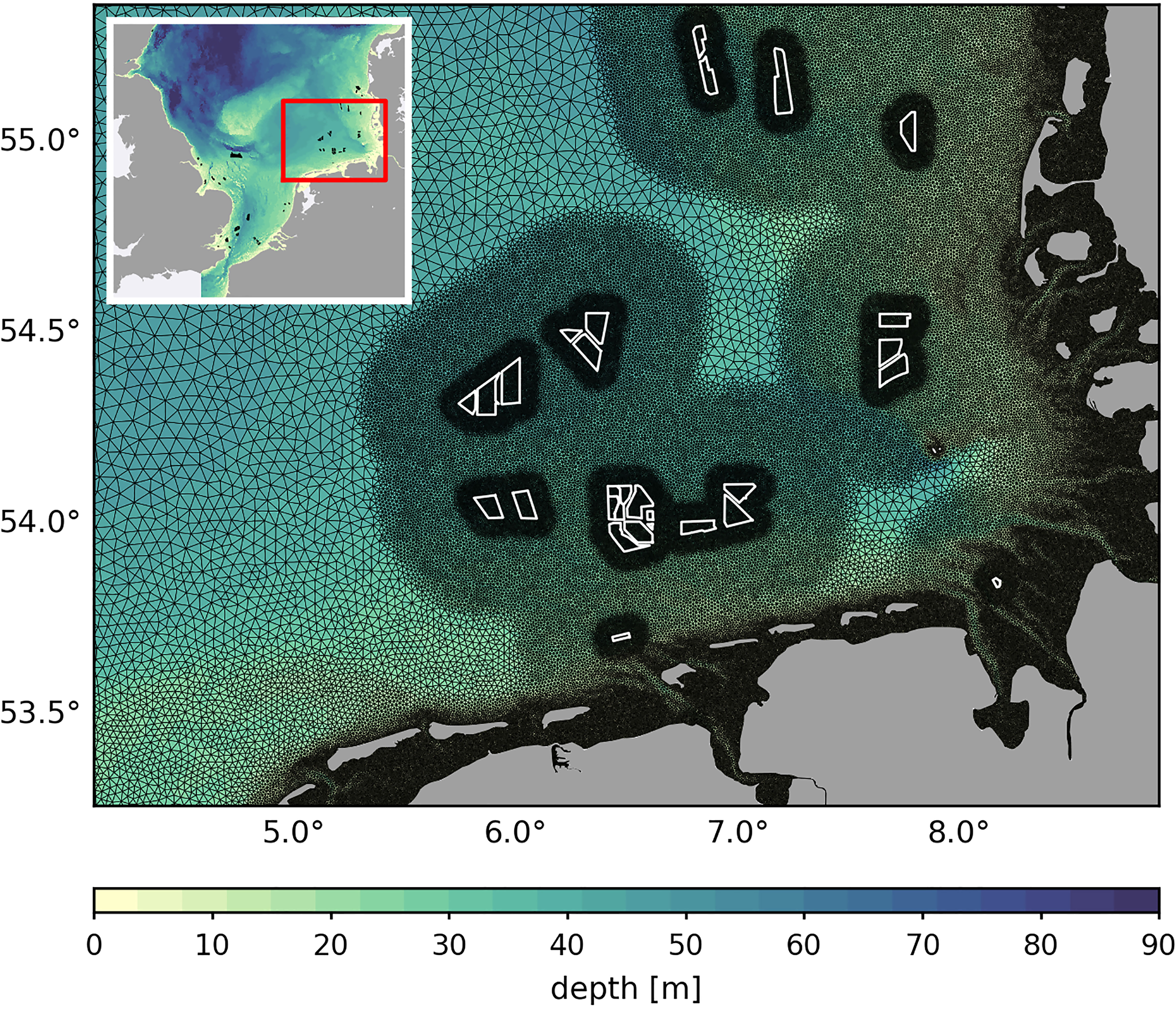
Figure 1 Horizontal grid resolution at offshore wind farms (white polygons) and near the coast. The entire model domain including all offshore wind farms used in this study (black polygons; data obtained from https://www.4coffshore.com/windfarms/) is shown in the top left corner.

At the lateral boundaries in the north and the southwest, horizontally and vertically interpolated daily means were prescribed for surface elevation, horizontal velocity, temperature and salinity from the North-West European shelf ocean physics reanalysis data from the Copernicus Marine Service (https://marine.copernicus.eu/, downloaded July 2019). In addition, tidal amplitudes and phases for eight tidal constituents (M₂, S₂, K₂, N₂, K₁, O₁, Q₁, P₁) from the HAMTIDE model (Taguchi et al., 2014) were applied at each time step of the simulation. For the atmospheric forcing, we used the coastDat-3 COSMO-CLM ERAinterim atmospheric reconstruction (HZG, 2017) and daily river discharge was provided by the mesoscale Hydrodynamic Model (mHM; Rakovec and Kumar, 2022). For more details about the model forcing and the model validation, see Christiansen et al. (2022).

Wake parameterization

The utilized model setup includes an empirical atmospheric wake parameterization based on satellite Synthetic Aperture Radar (SAR) data statistics and former wake models (Frandsen, 1992; Emeis and Frandsen, 1993; Frandsen et al., 2006; Emeis, 2010), which enables to reduce the surface wind speed u₀ on the lee side of offshore wind farms (Eq. (1)). The parameterization is defined as the wind speed recovery function u_r, describing the deficit in wind speed downstream of a wind farm. At this, the parameterization corresponds to a top-down approach, i.e. a wind farm is considered as a single unit.

The wakes are described by an exponential function in a reference coordinate system oriented along the prevailing wind direction. Here, x and y define the wind-aligned downstream distance and the distance from the central wake axis, respectively. The exponential function is determined by constant values describing the maximum percentage wind speed reduction (α), the scaling factor for the wake length (σ) and the scaling factor for the cross-sectional wake shape (γ). Values for α and σ were derived from SAR measurements at the offshore wind farm Global Tech and balanced by mean values of previous sea surface wake observations (Christiansen and Hasager, 2005; Christiansen and Hasager, 2006; Hasager et al., 2015; Djath et al., 2018; Djath and Schulz-Stellenfleth, 2019; Cañadillas et al., 2020). Although, magnitude and length of atmospheric wakes can vary strongly, depending on atmospheric conditions and wind farm configuration (Djath et al., 2018), the observation-based parameters give a sufficient estimate for the general impact of wind wakes, namely the downstream reduction in wind speed (see Christiansen et al., 2022). For α we used a constant value of 8%, whereas σ was set to 30 km. On the other hand, the scaling factor for the cross-sectional shape was calculated for each wind farm individually and is defined as γ = L/3, with L as the wind farm width with respect to the wind direction. The wake parameterization is applied to the wind field interpolated onto the model grid and reduces the wind speed at each time step of the model simulation. In this process, the horizontal velocity components at the downstream grid points of each wind farm are modified in the reference coordinate system, accordingly. A detailed description of the atmospheric wake parameterization is provided by Christiansen et al. (2022).

Model simulations

For the investigations of the tidal influence on wake-related processes, we applied four different simulations split into two scenarios: a tidal scenario (TIDES) and a tide-free scenario (NOTIDES). For each of the scenarios, we generated one reference simulation without wake parameterization (REF) and one simulation including the wake parameterization (OWF). Each simulation was calculated with an implicit time step of 120 seconds and produced hourly, instantaneous output data for the period of May to September 2013. The simulation period during the summer season was chosen to ensure mostly stable atmospheric conditions and to match the seasonal time span of the utilized satellite SAR measurements. For daily and monthly means, the absolute velocities were averaged over time. The NOTIDES scenario was generated using the same forcing data as for the TIDES, but without prescribing the amplitudes and phases of the different tidal constituents at the boundary nodes. For the wind farm simulations, the recent status (as of November 3, 2020) of offshore wind farm development in the North Sea was taken into account via the wake parameterization (data obtained from https://www.4coffshore.com/windfarms/). To illustrate the wake effects, the differences between the wind farm simulations to the reference simulations were used (OWF-REF).

Results and discussion

Primary wake effects

To investigate the impact of tides on processes related to the atmospheric wake effect, constant wind direction over at least one tidal period is beneficial, resulting in stable wake patterns. Here, we therefore focus on emerging wind wakes at offshore wind farms located in the Southern Bight, where the wind blows in northeasterly direction over a period of 48 hours between May 9 and May 11, 2013, nearly parallel to the local flood and ebb tide currents. As a result, stable wind speed reductions develop downwind, affecting the wind stress at the sea surface boundary and thus the horizontal surface velocity (Figure 2). In this context, wind speeds are on the order of about 10 m/s, whereas the tidal velocities range around 1 m/s, an order of magnitude lower. As the wind-driven horizontal currents are directly affected by the wind speed reduction, we define the induced changes in momentum and horizontal velocity as the primary wake effects. These effects do occur not only in the surface layer (Figures 2A, B), but are transferred to the entire water column (Figures 2C, D).

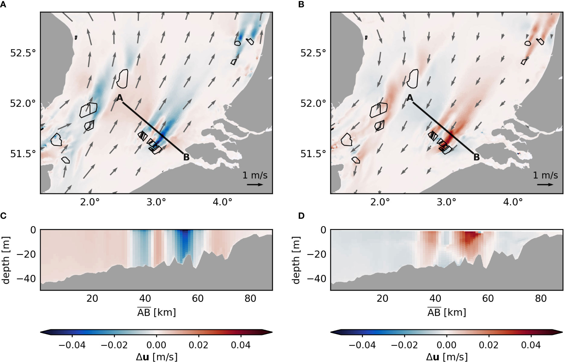
Figure 2 Horizontal velocity changes Δu in the tidal scenario (TIDES) during flood tide (A, C) and ebb tide (B, D). Flood and ebb tide examples correspond to May 10 at 03:00 and 09:00, respectively. Changes in horizontal velocity are shown for the surface layer (A, B) and with depth along the profile $\overline{\text{AB}}$ (C, D). Gray arrows indicate the direction of the horizontal tidal flow. Black polygons indicate the offshore wind farms.

Figure 2A shows the absolute changes in surface velocity during flood tide, where the tidal current flows in similar direction as the surface wind speed. As the reduced shear forcing leads to weaker wind-driven transport in the direction of the tidal current, the horizontal velocity decreases in the wake area, which is consistent with previous modeling studies (Ludewig, 2015; Christiansen et al., 2022). This process, however, cannot be generalized for the primary wake effects, as the induced changes in horizontal velocity appear to depend on the characteristics of the tidal flow. When the tidal cycle turns to ebb tide, wind field and tidal flow align in opposite directions (Figure 2B). In this case, the reduced shear forcing results in less countercurrents to the tidal current and thus the net transport along the wake area increases. Consequently, positive absolute changes develop in the wake area, contrary to the effects for aligned currents. Regardless of the alignment between wind and tides, the magnitudes of the wake-related horizontal velocity changes range between ±0.05 m/s, which accounts for about 5% of the maximum prevailing tidal velocities at the profile $\overline{\text{AB}}$, which range between 0.8-1.1 m/s during the selected time steps. As already mentioned by Christiansen et al. (2022), such strong velocity anomalies are substantial for the horizontal transport and persistent velocity perturbations due to the wind farms can influence the residual currents and the horizontal circulation.

In order to investigate how the relation between the wind direction and tidal flow determines the impact of atmospheric wind wakes, processes occurring over the entire tidal cycle of the example case are compared for the TIDES and NOTIDES scenarios. Figure 3 shows the temporal development of the absolute changes in wind speed and horizontal surface velocity as well as surface elevation and surface mixing between May 9 and May 11 along the profile $\overline{\text{AB}}$ roughly perpendicular to the mean wind direction (see Figure 2). During the two days, wind blows relatively constant from southwestern direction with an average wind speed of 10 m/s and a maximum of 15 m/s at the beginning of May 10 (Figure 3A). In the TIDES scenario, the average tidal flow along the profile changes with time according to its tidal ellipse, resulting in parallel and opposite flow directions between air and sea for flood and ebb tide, respectively (Figure 3A). The instantaneous tidal-driven surface currents averaged along profile $\overline{\text{AB}}$ are around 0.5 m/s. On the other hand, in the NOTIDES scenario horizontal currents are primarily wind-driven and therefore roughly parallel to the wind field over the selected period. Here, instantaneous surface currents range around 0.2 m/s. Opposing current directions, e.g. due to density-driven transport, are not evident during the selected period in the tide-free scenario.

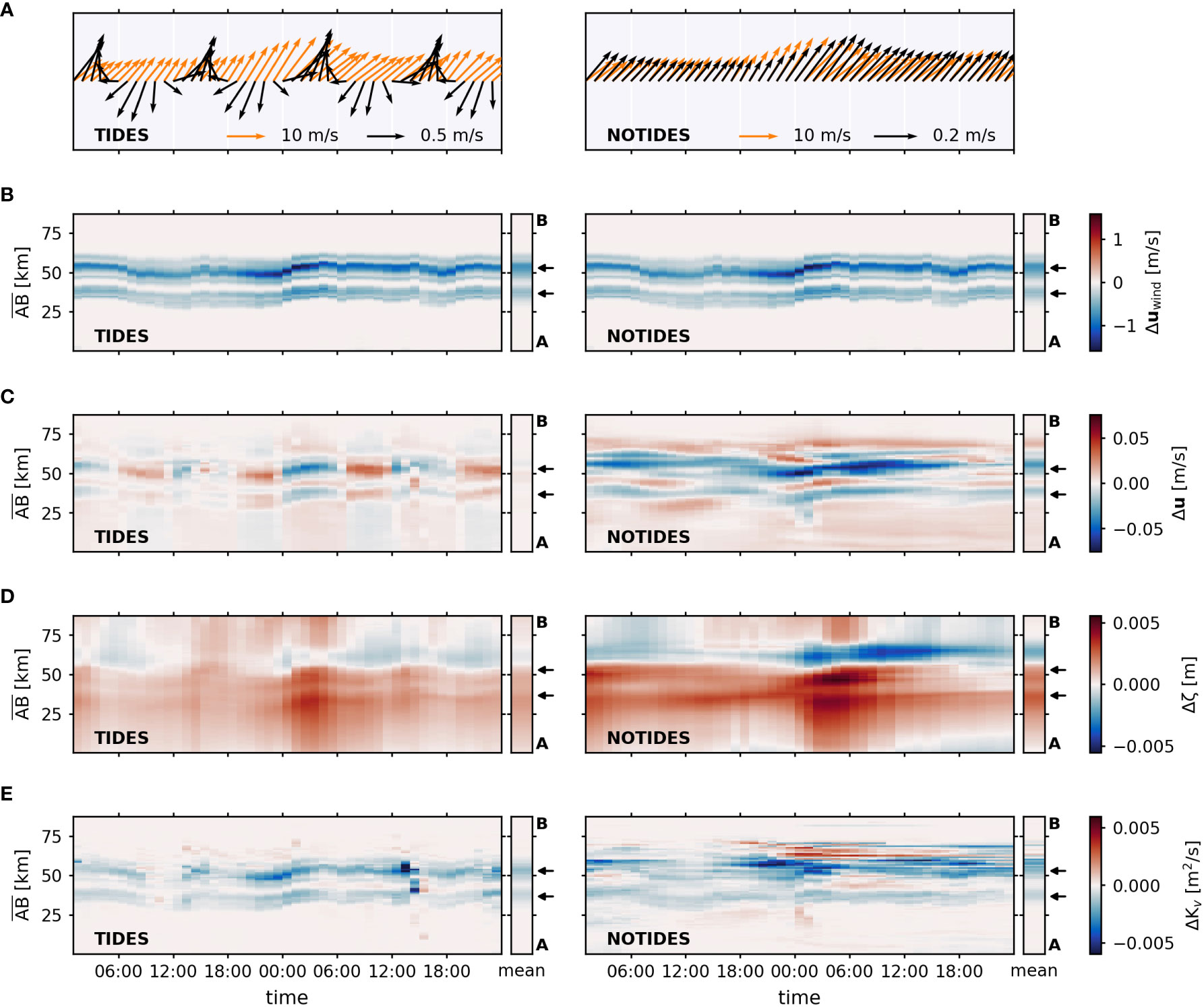
Figure 3 Wake effects along the profile $\overline{\text{AB}}$ (see Figure 2) for TIDES (left) and NOTIDES (right) between May 9 and May 11. (A) Vectors of the mean wind direction (orange) and the mean depth-averaged horizontal currents (black) along the profile, indicating the wind-ocean alignment. In addition, Hovmöller diagrams and temporal mean changes along profile $\overline{\text{AB}}$ are depicted for the relative differences in wind speed u (B), horizontal surface velocity u (C), sea surface elevation ζ (D) and surface eddy diffusivity K_v (E). Black arrows indicate the mean location of the wind wake maxima.

Figure 3C shows the response of the horizontal surface current to the wind speed reduction, i.e., the primary wake effect, and the role of the tidal flow on the emerging velocity anomalies. In TIDES, the horizontal velocity changes show the periodic change in amplitude and direction, which result from the periodic inversion of the tidal current. In this context, positive and negative velocity changes are directly related to the identified flow changes depicted in Figure 3A. The horizontal velocity changes in TIDES range between ±0.04 m/s, with the largest changes occurring on May 10 following the strong wind speed event and an average absolute change of about 0.025 m/s. While these changes account for about 1-5% of horizontal surface currents during tidal rise and fall (velocities between 0.6-1.2 m/s), they can account for more than 10% of horizontal surface currents at high and low tide (velocities between 0.1-0.3 m/s). However, the induced velocity changes do not affect the direction of the tidal flow or the tidal ellipses respectively. Due to the opposing effects, the mean changes over the 48-hour period are very small and show little effect on the mean horizontal flow compared to NOTIDES. Apparently, positive velocity changes due to countercurrents counteract the negative changes due to aligned currents and therefore prevent the development of consistent surface velocity reduction in TIDES. Consequently, the countercurrents attenuate the magnitude of the mean velocity anomalies along profile $\overline{\text{AB}}$. In this regard, mitigation depends on the consistency of the wind field and the ratio of the flood and ebb tide currents. In contrast, the NOTIDES scenario shows consistent reductions in surface velocity in the wake areas, which are also clearly visible on the 48-hour mean. Here, the instantaneous velocity changes are almost twice as strong as in TIDES with up to ±0.08 m/s and even account for about 50% of the actual horizontal wind-driven flow, implying significant changes in the tide-free scenario. The mean velocity changes reach up to ±0.025 m/s.

Secondary wake effects

Besides primary wake effects, atmospheric wakes trigger secondary effects associated to the primary changes in horizontal momentum and turbulence. Secondary wake effects involve, for instance, the reduction in wind-driven mixing of the surface layer due to weaker shear at the surface boundary (Christiansen et al., 2022) or the development of upwelling/downwelling dipoles due to changes in the Ekman dynamics (Broström, 2008; Paskyabi and Fer, 2012; Ludewig, 2015). Since primary and secondary wake effects are closely linked, the secondary effects are also expect to be attenuated by the inversion of the horizontal surface currents in TIDES.

Emerging sea level dipoles for both scenario are shown in Figure 3D. In NOTIDES, the consistent changes in horizontal surface velocity result in a pronounced dipole pattern along profile $\overline{\text{AB}}$, with magnitudes of induced sea level changes of about ±0.006 m. Mean changes are between ±0.0025 m. In contrast, the instantaneous and mean sea level changes in TIDES are again only half as strong as in NOTIDES, similarly to the horizontal velocity changes. Compared to the local tidal variability, the changes in sea surface elevation due to the wind speed reductions are insignificant for the tidal scenario. Here, the attenuation of the surface elevation dipoles results from the advection of the Ekman-related anomalies due to the variable tidal currents. The elliptical water parcel movement due to changing current directions continuously shifts the emerging anomalies around the actual location of the wind speed reduction, leading to a constant adjustment of the Ekman dynamics (see Supplementary Figure 1). Therefore, the periodic advection hinders the development of pronounced dipole maxima, causing an overall weaker dipole pattern along the wake axis compared to constant current direction. Periodic shifting of the surface elevation dipole can also be seen in Figure 3D. Nevertheless, a dipole pattern, albeit weaker, does still occur in TIDES for both instantaneous and mean sea surface height changes. Previous studies have shown that the wake-induced sea level dipoles are associated with changes in vertical transport and perturbations of the pycnocline (Broström, 2008; Paskyabi and Fer, 2012; Ludewig, 2015). Thus, attenuation of the sea level changes implies weaker changes in vertical velocities and density stratification. However, changes in vertical velocity are not clearly visible along profile $\overline{\text{AB}}$, since bathymetric features and strong tidal mixing impede the development of distinct wake-induced changes in the vertical velocity here. In addition to the sea surface elevation, changes in horizontal surface currents also affect the generation of turbulent kinetic energy and thus the turbulent mixing of the surface mixed layer. As the horizontal shear at the surface layer decreases with lower wind speeds, the vertical mixing rate decreases in the wake areas in both scenarios (Figure 3E). Here, we used the vertical eddy diffusivity K_v as a measure for the vertical mixing rate. Again, changes in the tidal scenario appear weaker over the 48-hour period. Particularly, during strong winds at the beginning of May 10, where the tidal direction is opposite to the wind direction, changes in mixing are clearly stronger in NOTIDES. Nevertheless, the order of magnitude of changes in eddy diffusivity is similar in TIDES and NOTIDES over time, especially along the wake at about 30 km of profile $\overline{\text{AB}}$, as the surface mixing is primarily determined by the wind stress. The magnitudes in TIDES are slightly lower on average due to the influence of tidal mixing. In both scenarios, the surface eddy diffusivity is reduced along the wind wakes by up to -0.006 m²/s and about -0.002 m²/s on average, indicating an enhancement of stratification in the surface layers along the wake areas. Temporarily, these changes can influence the actual eddy diffusivity in the surface layer (0.01-0.03 m²/s) significantly, especially in NOTIDES. However, compared to the depth-averaged eddy diffusivity, i.e., the tidal mixing in TIDES, the induced surface mixing reductions account for less than 10%.

Christiansen et al. (2022) showed that the magnitude of wake-induced stratification changes due to sea level dipoles or mixing reduction depend on the stratification conditions, suggesting a distinction between processes in stratified and well-mixed waters. To investigate this further, we analyze changes in vertical velocity and density gradients along profile $\overline{\text{CD}}$ northwards of the West and East Frisian Islands (Figure 4). Here, wake effects occur simultaneously in both stratified and mixed water. Again, we focus on a simulation period in which the wind remains stable over at least one tidal cycle. On May 2, winds blow constantly in southwesterly direction over a 12-hour period with mean wind speeds around 7 m/s (Figure 4A). During the period, the M2 tidal ellipses are mainly oriented in the direction of the wind field, but with deviations of up to 45 degrees. Three wake areas occur along the profile $\overline{\text{CD}}$ , resulting from offshore wind farms in the German Bight. The strongest wake-induced anomalies occur at a profile distance of about 80 km due to superposition of several emerging wakes behind the large wind farm cluster located at 54.0° N and 6.5° E (see Figure 4A). Another dominant wake pattern occurs at about 20 km. As shown before for profile $\overline{\text{AB}}$, constant wind direction and the periodic change of the tidal currents along profile $\overline{\text{CD}}$ result in opposing alterations of the horizontal surface currents and thus to perturbations of the secondary wake effects (see Figure 4D, C).

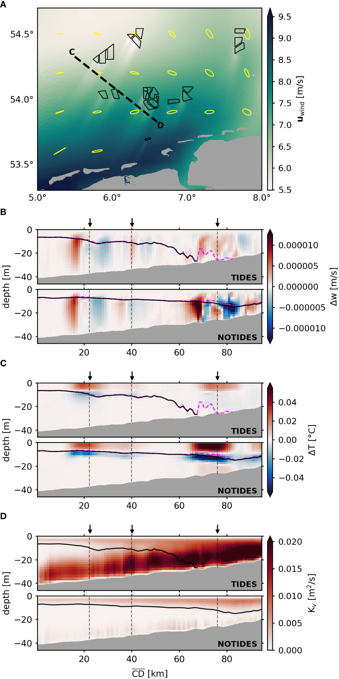
Figure 4 Mean wake effects along profile $\overline{\text{CD}}$ for TIDES and NOTIDES on May 2 between 06:00 and 18:00. (A) Mean wind speed u over the 12-hour period, illustrating the stable wake patterns in the example region. M2 tidal ellipses are indicated in yellow. Black polygons indicate the offshore wind farms. (B) Vertical profiles of the mean vertical velocity changes Δw over the 12-hour period in TIDES (top) and NOTIDES (bottom). Solid black line and dashed purple line show the mixed layer depth in the reference run (REF) and the wind farm run (OWF), respectively. Here, the mixed layer depth is defined by the density threshold criterion of Δρ = 0.03 kg/m³ (de Boyer Montégut et al., 2004). Arrows and black and gray dashed lines indicate mean location of wind wake maxima. (C) Vertical profiles of the mean temperature changes ΔT over the 12-hour period in TIDES (top) and NOTIDES (bottom). (D) Vertical profiles of the vertical eddy diffusivity K_v in the reference simulation (REF), indicating the mean vertical surface and bottom mixing rates in TIDES (top) and NOTIDES (bottom) over the 12-hour period.

Secondary wake effects influence the vertical velocity and density distribution through dipole-related vertical transport and the reduction of surface layer mixing. In this context, on the one hand, the latter results from the reduction in wind stress and leads to a general relaxation of the surface layers, which elevates the mean mixed layer depth and increases stratification strength in wake-affected areas (Figure 4B). The elevation of the mixed layer under the influence of wind wakes compared to the reference run is apparent in both TIDES and NOTIDES, affecting the temperature stratification near the surface mixed layer (Figure 4C). On the other hand, the sea level dipoles are associated with inverse changes in vertical transport, resulting in upwelling and downwelling patterns in the vertical velocity and stratification (Paskyabi and Fer, 2012; Ludewig, 2015). This is also shown here for the mean vertical velocity changes over the 12-hour period (Figure 4B). While these patterns can also lead to perturbations of the pycnocline, the upwelling/downwelling can affect the density distribution in the wake areas (Ludewig, 2015), which contributes to the occurring changes in mean temperature (Figure 4C).

In stratified deeper waters, distinct dipoles in the vertical velocity changes related to changes in Ekman transport are visible in regions influenced by wind speed reduction (Figure 4B). These dipoles occur similarly in TIDES and NOTIDES due to comparable stratification conditions and exhibit changes in mean vertical velocity of about ±7·10^-6 m/s. Consequently, similar changes in temperature stratification of about ±0.03°C occur in deeper waters (Figure 4C). In shallower regions, in contrast, induced changes differ significantly between TIDES and NOTIDES. In NOTIDES, the pycnocline persist in the shallow waters, allowing upwelling and downwelling patterns to continue to develop. The mean changes in the shallow waters exceed ±1·10^-5 m/s corresponding to approximately 1 meter per day, which agrees with the findings by Broström (2008) and Ludewig (2015). The vertical velocities as well as the reduced surface layer mixing result in distinct mean temperature changes of more than ±0.05°C. At this, magnitudes in velocity and temperature changes show a clear correlation with the magnitudes of the wind speed reduction.

In TIDES, however, the tidal mixing mitigates the secondary wake effects in shallow waters. Here, the strong vertical mixing rates from the bottom layers, which originate from tidal currents, overlap and dominate the wind-driven mixing from the surface layers (Figure 4D). As a result, the shallow waters in TIDES are well mixed and governed by tidal stirring. Consequently, Ekman dynamics are dominated by the strong tidal mixing rates and thus upwelling/downwelling is not visible in the vertical velocity changes along profile $\overline{\text{CD}}$ (Figure 4B). Besides, uniform vertical density distributions inhibits vertical transport in temperature and salinity. Instead, the induced changes in mean temperature stratification are primarily driven by the reduction of surface layer mixing, exhibiting magnitudes more than 50% weaker compared to NOTIDES (Figure 4C). At this, magnitudes do not appear related to the wind speed reductions, but to the extent of tidal influence. Hence, tidal mixing determines the impact of secondary wake effects on shallow coastal waters. In deeper waters, however, where the bottom shear and thus tidal mixing rates become less dominant, the secondary wake effects develop similarly in the tidal and non-tidal environment, particularly for increasing stratification strength.

Regional impact of tidal mitigation

According to the results of profiles $\overline{\text{AB}}$ and $\overline{\text{CD}}$, tides influence the wake effects on the hydrodynamics directly and indirectly through periodic currents and tidal mixing, respectively. The different tidal influences as well as primary and secondary wake effects are illustrated in Figure 5. On the one hand, the tidal currents have a direct impact on the surface velocity changes caused by the wind wakes, with frequently changing flow directions leading to deviations and inversions of the horizontal velocity changes (Figures 5A, B). In this context, both positive and negative instantaneous velocity changes can occur along the wake areas, as the reduction of wind stress reduces either the thrust of surface currents in tidal direction or the counterforce to the opposing tidal flow, depending on the alignment between wind and ocean current (see Figure 6A). Thus, direct tidal influences are related to the changes in vertical shear and affect particularly the wake-induced changes in the wind-driven flow and the mean horizontal circulation. With constant wind direction aligned with the tidal ellipses, the opposing changes in horizontal velocity at flood and ebb tide may even result in an attenuation of the mean velocity changes. Thus, the direct tidal influence can result in minor mean changes in horizontal velocity despite possibly strong instantaneous changes during the tidal cycle. This, however, requires equally strong flood and ebb currents and a constant wind field over the tidal cycle.

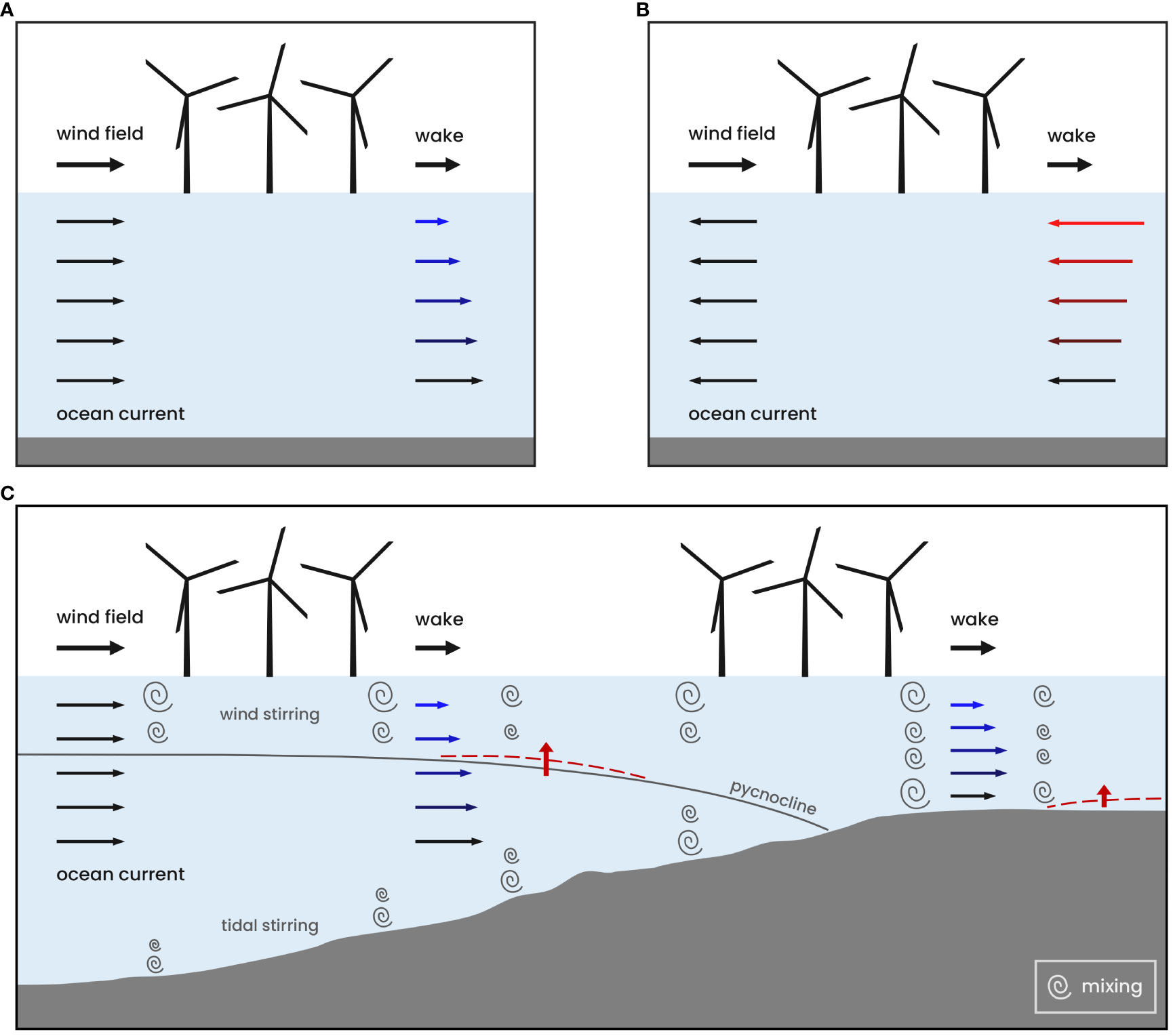
Figure 5 Schematic illustrations of tide-related hydrodynamic features (direct: periodic currents, indirect: mixing fronts) on the primary and secondary wake effects. (A) Primary wake effects, namely the reduction of the wind-driven ocean current, in the case of aligned wind and ocean currents. (B) Primary wake effects in the case of opposing wind and ocean currents. (C) Secondary wake effects, namely the mixing reductions and stratification increase, in stratified (left) and mixed (right) waters. Red dashed lines and arrows indicate the doming of the pycnocline in stratified waters and the development of a pycnocline in mixed waters, respectively.

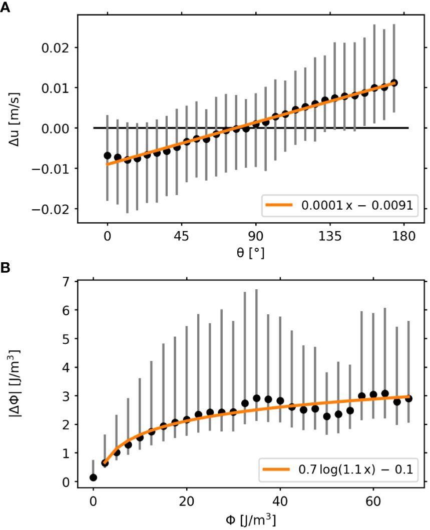
Figure 6 Correlations between the wind-tide alignment θ and the associated wind wake effects in horizontal velocity u (A), as well as between the potential energy anomaly Φ and associated absolute changes in potential energy anomaly Φ (B). The data points correspond to hourly data between May and August 2013, interpolated in areas of minimum 0.01 m/s wind speed reduction, and averaged in 5° bins and 2.5 J/m³ bins, respectively. Vertical gray lines show the standard deviation in each bin, whereas the orange lines show the respective fit of the mean changes per bin (black dots).

Regardless of the alignment between wind and tidal currents, the reduction in wind stress results in decreasing surface mixing and Ekman-driven vertical transport, ultimately affecting the pycnocline (Figure 5C). However, tidal mixing and stratification strength determine the magnitude of the secondary wake effects. This indirect impact of the tides occurs particularly in shallow waters where strong tidal stirring superimposes the surface layer mixing, hindering the development of Ekman-related vertical transport. In tidally dominated regions, therefore, secondary wake effects are limited to the reduction of surface layer mixing. Overall, wake-related changes in stratification appear as a function of the local stratification strength (see Figure 6B), which is governed by tidal mixing. In weakly stratified waters, secondary wake effects occur much weaker, whereas the mitigation effects diminish in more stratified deeper waters. Thus, local stratification strength can help to evaluate the expected impact of secondary wake effects.

It has been shown that the hydrodynamic effects of atmospheric wind farm wakes are not limited to local processes but involve large-scale structural changes in the hydrodynamic system (Christiansen et al., 2022). Thus, the influence of the tides must also be considered on regional scales. Figure 7 shows the regional mean changes in horizontal surface velocity and stratification strength over the entire simulation period between May and September. Both the changes for the scenario with (Figures 7A, C) and without tidal forcing (Figures 7B, D) are depicted. In TIDES, the changes in the mean surface currents show an inhomogeneous pattern with both positive and negative amplitudes around the wind farms (Figure 7A). This inhomogeneous pattern is related to the tidal influence during varying wind speeds and directions and unequal flood and ebb currents, resulting in positive, negative and deflected velocity changes over the period of five months. The velocity changes in the tidal scenario range between ±0.002 m/s. These changes are relatively small as they account for only about 0.5-1.0% of the actual mean horizontal surface velocities, which are between 0.2-0.5 m/s in the reference simulation. In contrast, the mean changes in NOTIDES are much larger (Figure 7B). Here, the changes are between ±0.01 m/s, which is an order of magnitude larger than in TIDES and accounts for about 5-10% of the mean horizontal velocities in the tide-free reference simulation, which are about 0.1-0.2 m/s. In addition, there are large-scale reductions in surface velocity around the wind farms, forming coherent patterns. Compared to TIDES, both the patterns and the magnitudes of the changes in NOTIDES clearly demonstrate the impact of the tidal currents on the primary wake effects. It shows that in highly tidal-driven environments, such as the southern North Sea, the mean changes in horizontal currents due to atmospheric wakes are attenuated and weaker than in the absence of tides. Nevertheless, we found that strong instantaneous changes, both positive and negative, still occur in the wake areas downstream of wind farms even in the tidal-driven environment, which can affect tidal stream transport and generation of turbulent mixing in the surface and bottom mixed layers. This becomes potentially important with regard to nutrient intrusion into the nutrient-depleted surface mixed layers (Schrum et al., 2006; Simpson and Sharples, 2012) or the larvae transport and fish migration (Gibson, 2003; van Berkel et al., 2020). In particular, the reduction of wind-driven surface layer mixing is not mitigated by the periodic flow reversals and thus can still affect stratification in the tidal environment.

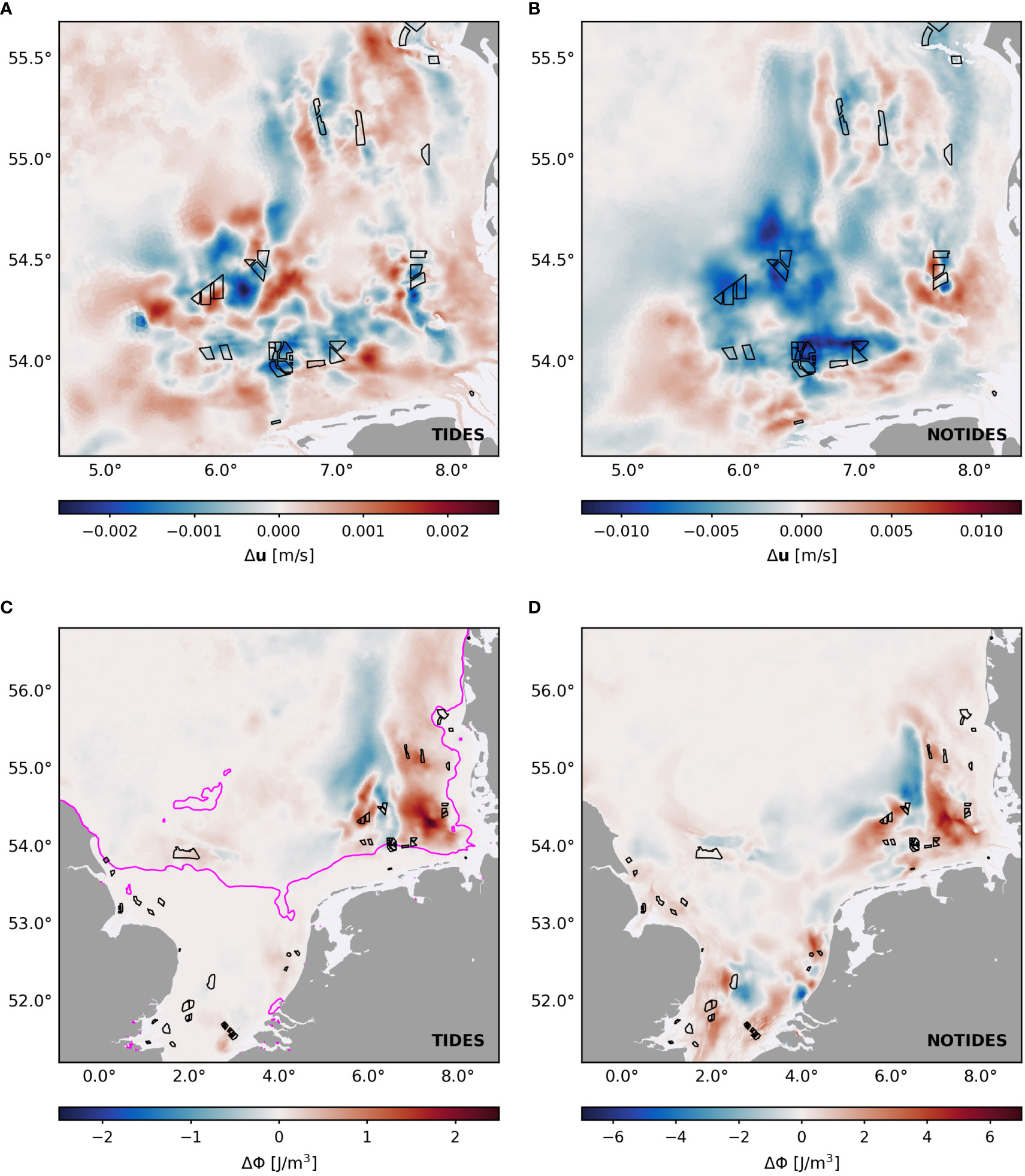
Figure 7 Regional mean wake effects on surface velocity u (A, B) and potential energy anomaly Φ (C, D) in TIDES (left) and NOTIDES (right). Monthly mean changes are depicted for the simulation period between May and September 2013. Magenta line in (C) indicates the mean tidal mixing fronts in TIDES. Black polygons indicate the offshore wind farms.

Despite impact on stratification in both scenarios, the influence of tides on secondary wake effects, specifically the changes in mean stratification, can be observed at the regional scale (Figures 7C, D). Here, changes in stratification are shown by changes in the potential energy anomaly, which is a gravitational-based measure of stratification strength (Simpson and Bowers, 1981). In TIDES, stratification changes occur mainly in the seasonally stratified regions and near the frontal areas of the southern North Sea, bounded by the location of the tidal mixing fronts (Figure 7C). Impact on weakly stratified waters is attenuated by strong tidal mixing rates. The changes in mean stratification strength range between ±2 J/m³, with a clear dipole pattern observed in the German Bight. This dipole pattern was shown to be related to the baroclinic changes and indicates an enhancement of the summer stratification towards the coastal waters (Christiansen et al., 2022). The NOTIDES scenario also shows a dipole pattern in the German Bight, indicating baroclinic changes (Figure 7D). In general, however, the changes in NOTIDES are more than twice as strong as in TIDES with values between ±5 J/m³, which is related to the overall stronger stratification in NOTIDES. At this, induced perturbations occur in all regions covered by wind farms, including significant stratification changes in the Southern Bight and regimes, which are characterized by strong mixing in the tidal environment. This clearly shows the influence of the tidal mixing on the development of the secondary wake effects.

With respect to the physical regimes of the southern North Sea, secondary wake effects appear to emerge primarily in seasonally and intermittently stratified regions, as tidal stirring in well-mixed regions mitigates the development of the wake effects. This becomes important regarding future expansion of offshore wind energy into deeper waters of the North Sea (WindEurope, 2022b). Based on the results, tidal mitigation will be minor in these regions and therefore the impact of the wind wakes on stratification will be more substantial. As Dorrell et al. (2022) noted, the effects of offshore wind farms in yet undeveloped areas have still to be investigated and could involve significant influence on the seasonal stratification. In terms of the wind farm effects, reduced surface layer mixing could further increase the stratification in wind farm areas. However, counteracting processes due to additional mixing from wind turbine foundations (see Carpenter et al., 2016; Schultze et al., 2020; Dorrell et al., 2022) could affect and even dominate the processes related to wind wakes. This leads to uncertainties about possible consequences in stratified waters, as the interaction of wind wake effects and additional turbulence inside the wind farm has yet to be determined. Furthermore, as shown by Christiansen el al. (2022), wake-related stratification changes also depend largely on induced sea level dipoles and could thus have both positive and negative amplitudes due to significant upwelling/downwelling patterns.

The tidal attenuation of vertical density stratification may mitigate not only the impact on the hydrodynamics in the southern North Sea but also impact on important ecological processes. Vertical mixing and stratification in the pycnocline are decisive factors in nutrient availability, primary production, and sediment resuspension (Sverdrup, 1953; Simpson and Sharples, 2012). Consequently, fluctuations of the mixed layer due to wake-related stratification changes are assumed to affect the nutrient balance in the system and thus primary production (Christiansen et al, 2022). van der Molen et al. (2014) simulated the effect of hypothetical wind speed reduction on biogeochemistry and, in fact, showed that the anomaly in wind speed resulted in higher ecosystem productivity and lower turbidity. With tidal mitigation, however, wind wake effects are much weaker and thus the potential impact on ecosystem dynamics. Nevertheless, van der Molen et al. also pointed out the counteracting processes of wind wakes and turbulent pile wakes and the need for further investigations, in order to evaluate the impact on the marine environment and determine the dominant processes.

Conclusion

Tides play an important role in the changes in hydrodynamics caused by atmospheric wind farm wakes. As our analysis showed, tides have both direct and indirect influences on the wake effects, altering the induced processes due to periodic tidal currents and tide-induced stratification conditions, respectively. While the tidal currents determine how the hydrodynamics respond to the wind speed reductions, stratification conditions and tidal mixing rates determine the impact on vertical transport and density stratification. In previous studies (Ludewig, 2015; Christiansen et al., 2022), the reduction of surface wind speed due to offshore wind farms has been associated to the reduction of the horizontal surface current. Here, however, we showed that tidal currents can deflect and even inverse wake-induced processes. Specifically, the alignment between wind and ocean currents determines the magnitudes of the wake effects. The periodic tidal currents can mitigate the impact of the wind speed reduction over time due to opposing changes in the horizontal flow, resulting in hydrodynamic changes only half as strong as those without tides. This mitigation can translate to secondary wake effects, like the development of sea level dipoles. However, we found that the degree of mixing in the water column is critical for the development of secondary wake effects, such as changes in vertical transport and density distribution. In this regard, induced changes are much more pronounced in stratified waters, whereas in well-mixed waters tidal stirring can influence the effects on vertical transport and attenuate the impact on temperature and salinity stratification.

In the southern North Sea, a tidal-driven environment, the strong tidal currents and the mixing induced by the tides appear to affect the wind wake effects on the hydrodynamics and even attenuate the induced mean changes. In this regard, our simulations suggest that the regional mean impacts in the southern North Sea would be more significant without tides. However, as the impact on the environment depends on the tidal and stratification conditions, the demonstrated attenuation of wake effects does not apply to all regions affected by offshore wind farm wakes. The Esbjerg Declaration 2022 (WindEurope, 2022a) as well as the EU’s renewable energy target of 40% by 2030 (WindEurope, 2022b) imply a significant expansion of offshore wind energy in European waters. These include the North Sea but also other marine environments characterized by different tidal regimes, water depths or stratification conditions. In the North Sea, an expansion of wind energy means development into seasonally stratified deeper waters with much lower tidal velocities (see Otto et al., 1990), such as the central or northeastern North Sea. In these regions, tidal mitigation effects will be weaker and wake effects, particularly the secondary wake effects that depend on stratification strength, may develop more strongly, suggesting stronger impact on vertical mixing and density stratification. On the other hand, primary wake effects might be much stronger in marine environments with almost no tidal energy, such as the Baltic Sea, where wind-driven processes are hardly affected by opposing ocean currents. The Baltic Sea, in particular, might be especially vulnerable to instantaneous and mean wind wake effects, as, in addition to mainly wind-driven and density-driven currents, salinity stratification persists throughout the year, complemented by seasonal temperature stratification (Leppäranta and Myrberg, 2009), and thus favors secondary wake effects. However, regional model simulations are needed to determine the actual response to wind wakes in these environments. Ultimately, we can say it is not only atmospheric conditions that determine the impact of atmospheric offshore wind farm wakes on the ocean, but also the regional hydrodynamic conditions in the respective environment. With this study, we emphasize the importance of the wind-tide interaction on the impact of wake effects on hydrodynamics and provide a guideline for wake effects in different marine environments.

Data availability statement

The raw data supporting the conclusions of this article will be made available by the authors on request.

Author contributions

NC generated the data set, performed the data analysis, and wrote the manuscript with input from all authors. UD and CS contributed to the data analysis and provided critical feedback. All authors contributed to the article and approved the submitted version.

Funding

This project is a contribution to the EXC 2037 ‘Climate, Climatic Change, and Society (CLICCS)’ (Project Number: 390683824) funded by the German Research Foundation (DFG), to the CLICCS-HGF networking project funded by the Helmholtz Association of German Research Centers (HGF), and to the Helmholtz Research Program “Changing Earth – Sustaining our Future”, Topic 4.

Conflict of interest

The authors declare that the research was conducted in the absence of any commercial or financial relationships that could be construed as a potential conflict of interest.

The reviewer TP declared a shared affiliation with the author CS to the handling editor at the time of review.

Publisher’s note

All claims expressed in this article are solely those of the authors and do not necessarily represent those of their affiliated organizations, or those of the publisher, the editors and the reviewers. Any product that may be evaluated in this article, or claim that may be made by its manufacturer, is not guaranteed or endorsed by the publisher.

Supplementary material

The Supplementary Material for this article can be found online at: https://www.frontiersin.org/articles/10.3389/fmars.2022.1006647/full#supplementary-material

References

Broström G. (2008). On the influence of large wind farms on the upper ocean circulation. J. Mar. Syst. 74, 585–591. doi: 10.1016/j.jmarsys.2008.05.001
Cañadillas B., Foreman R., Barth V., Siedersleben S., Lampert A., Platis A., et al. (2020). Offshore wind farm wake recovery: Airborne measurements and its representation in engineering models. Wind Energy 23, 1249–1265. doi: 10.1002/we.2484
Carpenter J. R., Merckelbach L., Callies U., Clark S., Gaslikova L., Baschek B. (2016). Potential impacts of offshore wind farms on north Sea stratification. PloS One 11, e0160830. doi: 10.1371/journal.pone.0160830
Christiansen N., Daewel U., Djath B., Schrum C. (2022). Emergence of Large-scale hydrodynamic structures due to atmospheric offshore wind farm wakes. Front. Mar. Sci. 9. doi: 10.3389/fmars.2022.818501
Christiansen M. B., Hasager C. B. (2005). Wake effects of large offshore wind farms identified from satellite SAR. Remote Sens. Environ. 98, 251–268. doi: 10.1016/j.rse.2005.07.009
Christiansen M. B., Hasager C. B. (2006). Using airborne and satellite SAR for wake mapping offshore. Wind Energy 9, 437–455. doi: 10.1002/we.196
de Boyer Montégut C., Madec G., Fischer A. S., Lazar A., Iudicone D. (2004). Mixed layer depth over the global ocean: An examination of profile data and a profile-based climatology. J. Geophys. Res. 109, C12003. doi: 10.1029/2004JC002378
Djath B., Schulz-Stellenfleth J. (2019). Wind speed deficits downstream offshore wind parks? A new automised estimation technique based on satellite synthetic aperture radar data. Meteorologische Z. 28, 499–515. doi: 10.1127/metz/2019/0992
Djath B., Schulz-Stellenfleth J., Cañadillas B. (2018). Impact of atmospheric stability on X-band and c-band synthetic aperture radar imagery of offshore windpark wakes. J. Renewable Sustain. Energy 10, 43301. doi: 10.1063/1.5020437
Dorrell R. M., Lloyd C. J., Lincoln B. J., Rippeth T. P., Taylor J. R., Caulfield C.-c. P., et al. (2022). Anthropogenic mixing in seasonally stratified shelf seas by offshore wind farm infrastructure. Front. Mar. Sci. 9. doi: 10.3389/fmars.2022.830927
Emeis S. (2010). A simple analytical wind park model considering atmospheric stability. Wind Energy 13, 459–469. doi: 10.1002/we.367
Emeis S., Frandsen S. (1993). Reduction of horizontal wind speed in a boundary layer with obstacles. Boundary-Layer Meteorology 64, 297–305. doi: 10.1007/BF00708968
Emeis S., Siedersleben S., Lampert A., Platis A., Bange J., Djath B., et al. (2016). Exploring the wakes of large offshore wind farms. J. Physics: Conf. Ser. 753, 92014. doi: 10.1088/1742-6596/753/9/092014
Frandsen S. (1992). On the wind speed reduction in the center of large clusters of wind turbines. J. Wind Eng. Ind. Aerodynamics 39, 251–265. doi: 10.1016/0167-6105(92)90551-K
Frandsen S., Barthelmie R., Pryor S., Rathmann O., Larsen S., Højstrup J., et al. (2006). Analytical modelling of wind speed deficit in large offshore wind farms. Wind Energy 9, 39–53. doi: 10.1002/we.189
Gibson R. (2003). Go with the flow: tidal migration in marine animals. Hydrobiologia 503, 153–161. doi: 10.1023/B:HYDR.0000008488.33614.62
Hasager C. B., Vincent P., Badger J., Badger M., Di Bella A., Peña A., et al. (2015). Using satellite SAR to characterize the wind flow around offshore wind farms. Energies 8, 5413–5439. doi: 10.3390/en8065413
HZG (2017). “coastDat-3_COSMO-CLM_ERAi,” in World data center for climate (WDCC) at DKRZ. Available at: http://cera-www.dkrz.de/WDCC/ui/Compact.jsp?acronym=coastDat-3_COSMO-CLM_ERAi.
Leppäranta M., Myrberg K. (2009). Physical oceanography of the Baltic Sea (Berlin, Heidelberg: Springer). doi: 10.1007/978-3-540-79703-6_3
Li X., Lehner S. (2013). Observation of TerraSAR-X for studies on offshore wind turbine wake in near and far fields. IEEE J. Selected Topics Appl. Earth Observations Remote Sens. 6, 1757–1768. doi: 10.1109/JSTARS.2013.2263577
Lissaman P. B. S. (1979). Energy effectiveness of arbitrary arrays of wind turbines. J. Energy 3, 323–328. doi: 10.2514/3.62441
Ludewig E. (2015). On the effect of offshore wind farms on the atmosphere and ocean dynamics (Springer International Publishing: Cham). doi: 10.1007/978-3-319-08641-5
Otto L., Zimmerman J., Furnes G. K., Mork M., Saetre R., Becker G. (1990). Review of the physical oceanography of the north Sea. Netherlands J. Sea Res. 26, 161–238. doi: 10.1016/0077-7579(90)90091-T
Paskyabi M. B., Fer I. (2012). “Upper ocean response to Large wind farm effect in the presence of surface gravity waves,” in Selected papers from Deep Sea Offshore Wind R&D Conference. (Trondheim, Norway) 24, 245–254. doi: 10.1016/j.egypro.2012.06.106
Platis A., Bange J., Bärfuss K., Cañadillas B., Hundhausen M., Djath B., et al. (2020). Long-range modifications of the wind field by offshore wind parks? Results of the project WIPAFF. Meteorologische Z. 29, 355–376. doi: 10.1127/metz/2020/1023
Platis A., Hundhausen M., Mauz M., Siedersleben S., Lampert A., Bärfuss K., et al. (2021). Evaluation of a simple analytical model for offshore wind farm wake recovery by in situ data and weather research and forecasting simulations. Wind Energy 24, 212–228. doi: 10.1002/we.2568
Platis A., Siedersleben S. K., Bange J., Lampert A., Bärfuss K., Hankers R., et al. (2018). First in situ evidence of wakes in the far field behind offshore wind farms. Sci. Rep. 8, 2163. doi: 10.1038/s41598-018-20389-y
Rakovec O., Kumar R. (2022). “Mesoscale hydrologic model based historical streamflow simulation over Europe at 1/16 degree,” in World data center for climate (WDCC) at DKRZ. doi: 10.26050/WDCC/mHMbassimEur
Schrum C., Alekseeva I., St. John M. (2006). Development of a coupled physical-biological ecosystem model ECOSMO part I: model description and validation for the north Sea. J. Mar. Syst. 61, 79–99. doi: 10.1016/j.jmarsys.2006.01.005
Schultze L. K. P., Merckelbach L. M., Horstmann J., Raasch S., Carpenter J. R. (2020). Increased mixing and turbulence in the wake of offshore wind farm foundations. J. Geophys. Res. Oceans 125, e2019JC015858. doi: 10.1029/2019JC015858
Siedersleben S. K., Platis A., Lundquist J. K., Lampert A., Bärfuss K., Cañadillas B., et al. (2018). Evaluation of a wind farm parametrization for mesoscale atmospheric flow models with aircraft measurements. Meteorologische Z. 27, 401–415. doi: 10.1127/metz/2018/0900
Simpson J. H., Bowers D. (1981). Models of stratification and frontal movement in shelf seas. deep Sea research part a. Oceanographic Res. Papers 28, 727–738. doi: 10.1016/0198-0149(81)90132-1
Simpson J. H., Sharples J. (2012). Introduction to the physical and biological oceanography of shelf seas (Cambridge: Cambridge University Press). doi: 10.1017/CBO9781139034098
Sündermann J., Pohlmann T. (2011). A brief analysis of north Sea physics. Oceanologia 53, 663–689. doi: 10.5697/oc.53-3.663
Sverdrup H. U. (1953). On conditions for the vernal blooming of phytoplankton. ICES J. Mar. Sci. 18, 287–295. doi: 10.1093/icesjms/18.3.287
Taguchi E., Stammer D., Zahel W. (2014). Inferring deep ocean tidal energy dissipation from the global high-resolution data-assimilative HAMTIDE model. J. Geophys. Res. Oceans 119, 4573–4592. doi: 10.1002/2013JC009766
van Berkel J., Burchard H., Christensen A., Mortensen L. O., Svenstrup Petersen O., Thomsen F. (2020). The effects of offshore wind farms on hydrodynamics and implications for fishes. Oceanography 33, 108–117. doi: 10.5670/oceanog.2020.410
van der Molen J., Smith H. C., Lepper P., Limpenny S., Rees J. (2014). Predicting the large-scale consequences of offshore wind turbine array development on a north Sea ecosystem. Continental Shelf Res. 85, 60–72. doi: 10.1016/j.csr.2014.05.018
van Leeuwen S., Tett P., Mills D., van der Molen J. (2015). Stratified and nonstratified areas in the north Sea: Long-term variability and biological and policy implications. J. Geophys. Res. Oceans 120, 4670–4686. doi: 10.1002/2014JC010485
Wilson R. E. (1980). Wind-turbine aerodynamics. Wind Energy Conversion Syst. 5, 357–372. doi: 10.1016/0167-6105(80)90042-2
WindEurope (2021). Offshore wind in Europe: Key trends and statistics in 2020. Available at: https://windeurope.org/intelligence-platform/product/offshore-wind-in-europe-key-trends-and-statistics-2020/.
WindEurope (2022a) The esbjerg offshore wind declaration: The north Sea as a green power plant of Europe. Available at: https://windeurope.org/policy/joint-statements/the-esbjerg-offshore-wind-declaration/.
WindEurope (2022b) Wind energy in Europe: 2021 statistics and the outlook for 2022-2026. Available at: https://windeurope.org/intelligence-platform/product/wind-energy-in-europe-2021-statistics-and-the-outlook-for-2022-2026/.
Keywords: tides, mitigation, offshore, wind farms, wakes, North Sea
Citation: Christiansen N, Daewel U and Schrum C (2022) Tidal mitigation of offshore wind wake effects in coastal seas. Front. Mar. Sci. 9:1006647. doi: 10.3389/fmars.2022.1006647
Received: 29 July 2022; Accepted: 20 September 2022;
Published: 03 October 2022.
Edited by:
Alejandro Jose Souza, Center for Research and Advanced Studies - Mérida Unit, MexicoReviewed by:
Robert Dorrell, University of Hull, United KingdomThomas Pohlmann, University of Hamburg, Germany
Copyright © 2022 Christiansen, Daewel and Schrum. This is an open-access article distributed under the terms of the Creative Commons Attribution License (CC BY). The use, distribution or reproduction in other forums is permitted, provided the original author(s) and the copyright owner(s) are credited and that the original publication in this journal is cited, in accordance with accepted academic practice. No use, distribution or reproduction is permitted which does not comply with these terms.
*Correspondence: Nils Christiansen, nils.christiansen@hereon.de