Estimates of Methane Release From Gas Seeps at the Southern Hikurangi Margin, New Zealand

Introduction

Methane forms in marine sediments that are rich in organic matter through either microbial methanogenesis or thermogenic processes (Schoell, 1988). Methane formation occurs at different depths in the subsurface but, because of the buoyancy of the gas, it migrates upwards through pathways that include permeable carrier sedimentary units, faults, or densely fractured regions (Cook and Malinverno, 2013; Crutchley et al., 2015; Nole et al., 2016; Hillman et al., 2017; Hoffmann et al., 2019; Hillman et al., 2020). When these pathways connect to the surface, gas bubbles escape the seafloor as gas seeps, which can range from diffusive sporadic and localized emanations of bubbles to widespread, vigorous gas seeps, occurring in different geological contexts, from the coastal environments to deep ocean regions (Judd, 2004; Duarte et al., 2007; Watson et al., 2020). In shallow waters—up to 800 mbsl, the gas bubbles can reach the sea surface and release greenhouse gases into the atmosphere (Schmale et al., 2005), having direct implications for climate. In deeper seas, however, most of the gas that is released at the seabed dissolves into the ocean without reaching the sea surface, causing localized methane-induced seawater acidification over long time scales (Law et al., 2010; Biastoch et al., 2011; Garcia-Tigreros et al., 2021).

Seismic and acoustic methods are useful tools to identify, map and characterize free gas accumulations in the subsurface (e.g., Judd and Hovland, 1992; Kim et al., 2020), evidence for past and present seepage at the seafloor (e.g., Stott et al., 2019) and gas release into the water column (e.g., Colbo et al., 2014; Böttner et al., 2020). In the subsurface, the presence of gas in the pore-space significantly affects the elastic properties of the bulk sediment, primarily by reducing the bulk seismic velocities and generating a contrast in acoustic impedance. The detection, mapping and characterization of subsurface gas reservoirs are parts of the traditional hydrocarbon exploration workflow (Yilmaz, 2001). Low seismic velocities, often associated with fluid migration through geological structures such as chimneys, conduits, and faults, can be an indicator of free gas in the sediments.

In the ocean, columns of rising gas bubbles (also called flares for the typical shape they assume in hydroacoustic imaging) are less dense than seawater and thus represent strong acoustic reflectors, as they generate sharp localized changes in the acoustic impedance of the water column. Calculating methane fluxes at a seep site is challenging, as it requires ground-truth information about bubble size distribution, chemical composition, density, bubble coating, and ascending speed (Leblond et al., 2014). Typically, gas bubbles released at the seafloor tend to have a radius in the range of 1–15 mm (Veloso et al., 2015), resonating at frequencies from a few hundred Hz to ∼12 kHz, depending on depth and size (Weidner et al., 2019). Single-frequency sonar systems have been successfully used for the identification of seep sites and for water column imaging for decades (e.g., Merewether et al., 1985; Hornafius et al., 1999; Nikolovska et al., 2008). However, these instruments cannot be used to determine the size distribution of the bubble population.

A common approach for the estimation of gas fluxes is coupling acoustic imaging of the gas bubbles with optical point-source measurements from towed camera systems (Higgs et al., 2019), remotely operated vehicles (Naudts et al., 2010), bubble observation modules (Bayrakci et al., 2014) or bubble traps (Römer et al., 2012). Although these point-source measurements provide the most accurate observation of bubble parameters, they require long deployment durations and a restricted field of view of less than ∼15 m. Moreover, they are also limited to measurements at the seafloor, and cannot provide a way to track the changes in bubble size distribution as they rise through the water column. Broadband hydroacoustic methods provide a more efficient tool to directly estimate bubble parameters by insonifying large areas of the oceans using a range of frequencies (e.g., Veloso et al., 2015; Colbo et al., 2014; Dupré et al., 2015; von Deimling et al., 2011; Li et al., 2020).

The highest concentration of cold seep sites worldwide has been observed along convergent margins, (Saffer and Tobin, 2011; Suess, 2020; Watson et al., 2020). In these regions, gas flares observed at the seabed and other shallow gas migration features are often connected to subsurface methane reservoirs through gas conduits (e.g., Meldahl et al., 2001; Petersen et al., 2010; Krabbenhoeft et al., 2013; Crutchley et al., 2021). On the seafloor, gas seeps are the most common manifestations of ongoing subsurface fluid flow (Judd and Hovland, 2009). The gases that are expelled from gas seeps on continental margins are primarily composed of methane, leaving major questions open on: 1) the amount of methane reaching the ocean surface (McGinnis et al., 2006; Shakhova et al., 2010; Fu et al., 2020), 2) the connectivity of seeps to deeper hydrocarbon systems (Crutchley et al., 2021), 3) the role of gas hydrate dissociation (Reagan et al., 2011), 4) how gas flux rates change over time and the potential influence of seismicity on subsurface fluid flow (Bassett et al., 2014; Bonini, 2019; Legrand et al., 2021). The southern Hikurangi Margin, off the North Island of Aotearoa/New Zealand, reveals evidence of widespread methane seepage (Greinert et al., 2001; Barnes et al., 2010; Watson et al., 2020). The accretionary wedge here consists of a series of thrust-related ridges striking NE-SW, composed of compressed and deformed sediments, probably turbidites and ancient trench-fill deposits (Kroeger et al., 2015; Lewis et al., 1998). Seismic data show evidence of concentrated gas hydrate accumulations in the core regions of many thrust ridges in this region, indicating the preferential migration of free gas along permeable strata towards the core of anticlinal structures (Crutchley et al., 2019; Turco et al., 2020; Wang et al., 2017a; Schwalenberg et al., 2010; Kroeger et al., 2021). Estimation of gas fluxes at gas seeps on the Hikurangi Margin has so far relied on in situ optical measurements of gas bubbles (Naudts et al., 2010; Higgs et al., 2019) combined with single-beam acoustic data.

In this paper, we use a combination of seismic and acoustic data to characterize five known sites of active gas seepage on the southern Hikurangi Margin. The interpretation of seismic amplitudes provides a means to identify regions of free gas accumulations within the sediments. Qualitative analysis of multibeam data collected over 3 years allows the spatial extent of the region of active venting at the seafloor to be mapped, while also imaging the acoustic flares in the water column and analyzing their variability over time. Split-beam echo sounder data are used to extract important parameters for the quantification of gas bubbles in the water from the backscattered acoustic energy, which are then used to calculate gas fluxes at the cold seep locations.

Data and Methods

Acoustic Data Processing

The identification and mapping of gas seeps in deep waters was achieved through the analysis of acoustic data (Figure 1). Bathymetric and water column data were acquired during three scientific voyages onboard the R/V Tangaroa (Figure 2): TAN1808 (September-October 2018), TAN1904 (July 2019) and TAN2012 (November 2020).

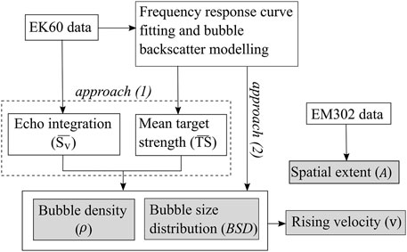
FIGURE 1. Illustration of the workflow to estimate gas fluxes from MBES (EM302) and single-beam (EK60) backscatter data. Approach (1) is based on the manual curve fitting of the normalized frequency response of the 18 and 38 kHz channels of the EK60 data, while approach (2) is based on a linear inversion of the non-normalized frequency response. S_v, mean volume backscattering strength computed for each cell; $\overline{\mathit{TS}}$, mean target strength computed for the whole acoustic flare; ρ, density of bubbles; BSD, bubble size distribution; v, bubble rising velocity; A, spatial extent of acoustic anomaly.

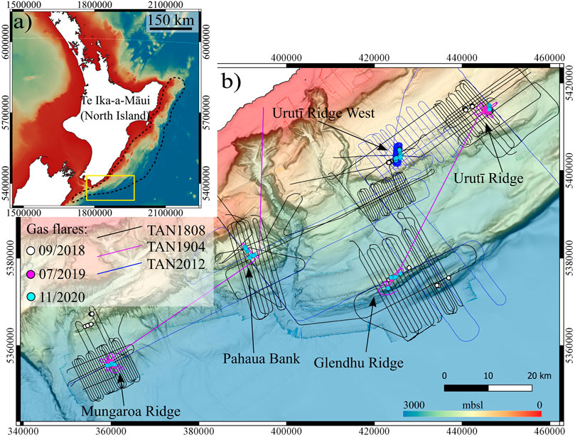
FIGURE 2. (A) Overview of the Hikurangi subduction Margin of New Zealand (dashed black line) and the study area (yellow rectangle). (B) expansion of the study area on the southern Hikurangi Margin: white, cyan and magenta dots are gas flares identified from the MBES data from the three R/V Tangaroa voyages (TAN1808, TAN1904, TAN2012). The five target areas are mentioned in the text. Map coordinates are in metres of New Zealand Transverse Mercator 2000 (New Zealand Geodetic Datum 2000).

Swath bathymetry and acoustic backscatter of mid-water reflectors were collected with a hull-mounted Kongsberg EM302 multibeam echo-sounder during the three voyages. The EM302 echo sounder operates at a nominal frequency of 30 kHz and with a swath of ∼120°. The use of the multibeam data was twofold: 1) to accurately locate gas seeps on the seafloor and 2) to calculate the area of seepage at the seafloor. For the former objective, the data were processed using the National Institute of Water and Atmospheric Research (NIWA) custom-built software Espresso with the following steps: seafloor detection filtering, removal of the outermost noisy beams (>45°), removal of bad pings, filtering side lobe artefacts and muting the first 5 m of data above the automatically picked seafloor, to avoid misinterpreting the smearing of the beams at the seafloor as gas bubbles (Schimel et al., 2020). The correct pinpoint (as well as could be determined) of seepage at the seafloor was facilitated by the fan visualization of MBES data (Figure 3). To calculate the total area of gas seepage in proximity of the seafloor, the processed data were vertically summed over a window between 5 and 20 m above the seabed - a process known as echo integration (MacLennan et al., 2002). The output of this process is a georeferenced image of volume backscatter intensity with a horizontal spatial resolution of 15 m × 15 m, that allowed mapping the spatial extent of the acoustic anomaly in the water column.

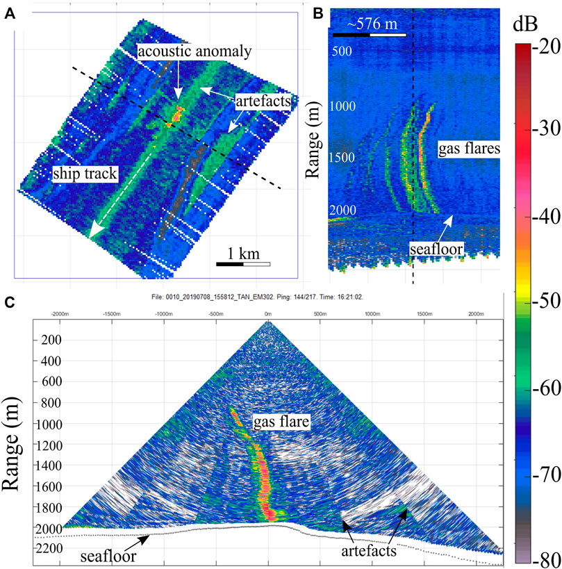
FIGURE 3. Backscatter intensity images of the Glendhu seep field (see Figure 2 for location) from multibeam data. (A) echo integrated map (resolution 20 × 20 m); (B) range stacked view along the profile shown in a); (C) fan view at the location indicated by the dashed black line in (A).

A suite of 5 Simrad EK60 echo sounders were used to obtain calibrated acoustic measurements of the water column during TAN1904 and TAN2012 voyages. The data were acquired over the five targeted areas based on existing multibeam coverage. These split-beam systems were calibrated using a standard 38.1 mm tungsten sphere hung under the vessel, following standard procedures (Demer et al., 2015). Given the relatively great water depth of most targeted flares (>1,000 mbsl), only the 18 and the 38 kHz echo sounders had sufficient range to image the full vertical extent of the gas bubbles. The two-way beam angle of the EK60 echo sounder is 11° for the 18 kHz system and 7° for the 38 kHz one. We extracted and processed the data recorded for the targeted gas flares using the open-source software package ESP3 (Ladroit et al., 2020). The data were processed to only extract the acoustic signal associated with gas venting. The processing included seafloor echo detection and removal, bad ping removal and de-noising (De Robertis and Higginbottom, 2007). Once acoustic flares were identified and extracted, we carried out frequency analysis on the pre-processed split-beam data and compared the frequency response to theoretical bubble backscatter models to estimate the bubble size distribution (BSD) of the entire flare (Figure 1). Finally, we echo integrated the processed 18 kHz data using cells 25 m high and 10 m wide, in order to retrieve a mean volume backscattering strength ($\overline{S_v}$) response for each cell.

Estimation of Gas Fluxes

Existing theoretical models to predict the acoustic backscattering cross-section (${\sigma }_{bs})$ of underwater bubbles differ in terms of parameters such the bubble size distribution (BSD), bubble morphology, the frequency range of the acoustic signal and the environment characteristics. For the scope of this work, we adopt the model proposed by Ainslie and Leighton (2009). For a more complete overview of the definitions and terminology used in underwater acoustics and adopted in this work the reader is referred to, e.g., MacLennan et al. (2002).

The workflow to estimate gas fluxes at the seep locations is illustrated in Figure 1. To estimate the BSD and density, we followed two approaches, one based on the normalized frequency response of the 18 and 38 kHz channels of the EK60 data, and one based on the non-normalized frequency response, similarly to the approach used by Li et al. (2020).

In the first approach (1), gas flares were isolated using the 18 kHz data, and they were echo integrated using a variable cell size ranging from 25–50 m in height and 5–10 m in width. The echo integration process yields a mean volume backscattering strength ($\overline{S_v}$) for each cell of the acoustic flare. The frequency analysis of the gas plume from both the 18 and 38 kHz channels, normalized relatively to the 38 kHz $S_v$ values, provides frequency-dependent $S_v$ values that the theoretical backscatter model curves aim to match. The curve-matching procedure was achieved through manual tuning of the mean bubble radius and bubble size distribution. When the match is considered satisfactory, i.e., when the residuals between the observed and the theoretical $S_v$ are below a chosen threshold for each water depth, the resulting BSD is considered representative of the entire flare, and the mean backscattering cross-section is computed following:

where $BSD$ is the bubble size distribution, and $a$ the bubble radius. ${\sigma }_{bs}$ is given byAinslie and Leighton (2009):

where $\omega$ is the frequency of the active source of the acoustic signal, ${\omega }_1$ is the resonance frequency of the bubble and $\delta$ is a dimensionless frequency-dependant damping constant. To retrieve the density of bubbles per volume unit, the mean volume backscattering strength $\overline{S_v}$ value of each cell of the echo integrated flare is compared to the representative mean target strength ($\overline{TS}$) value of the whole flare. Eq. 3 relates the mean backscattering cross-section representative of the entire flare $\overline{{\sigma }_{bs}}$ (in m⁻¹, or expressed in decibels by $\overline{TS}$) to the mean volume backscattering coefficient of a given cell of the echogram $\overline{s_v}$ (m², or $\overline{S_v}$ in decibels), following:

Then, $\rho$ is averaged across cells located at the same water depth, hence a mean density of bubbles is estimated for each horizontal slice of the gas flare ($\overline{\rho }$).

The second approach (2) to retrieve BSD and $\overline{\rho }$ for each flare consists of a linear inversion technique that aims to minimize the difference between the modelled and the observed non-normalized volume scattering strengths at each depth of the acoustic flare. The forward modelled data are computed following the theoretical backscatter model by Ainslie and Leighton (2009), and the optimization is achieved through a conjugate gradient technique. The model parameters that are inverted are bubble size, bubble size distribution parameters (for a fixed distribution type) and density of bubbles per volume unit. These parameters are initialized using the results from the first approach and updated iteratively during the inversion. 100 iterations were performed on each flare, and the inversion was carried out twice, once assuming a log-normal type bubble size distribution (Veloso et al., 2015), and once assuming a Weibull type distribution (Dey and Kundu, 2012).

Once the BSD and $\overline{\rho }$ are known, the gas flux is estimated for the entire flare (which could represent a field of seeps) following Eq. 4:

where $A$ is the spatial extent of the acoustic anomaly in the proximity of the seafloor as interpreted from the processed MBES data, $\overline{\rho }$ is the mean density of bubbles in the water in m⁻³, $\text{v}\left(\text{a}\right)$ is the mean rising velocity of the gas bubbles, $BSD$ is the bubble size distribution and $a$ is the bubble radius. The bubble rise velocity valuesare based on the work by Leifer and Patro (2002) and consider the two endmembers clean and coated bubbles, where the latter model represents gas bubbles which are coated with oil or hydrate (Fu et al., 2020).

In the next section, the estimated gas fluxes are presented as ranges of values. The major source of variability in the flux estimations comes from the use of coated versus clean bubbles models: because clean bubbles rise faster than coated bubbles, changes in $\text{v}$ have a linear effect on the fluxes (Eq. 4). Hydrate-coated bubbles have been observed at some of the seep sites analyzed in this paper (Sarah Seabrook, personal communication). However, due to the scarcity of observational data, we use both models to provide a range of possible gas flux estimates.The secondary source of uncertainty in the estimations is related to the approach used for the calculation of the $BSD$ and density (Figure 1). These parameters impact both the mean rising velocity–which depends on the bubble size, and the volume of gas calculated at the seafloor.

Because of the lack of in situ chemical measurements at the locations of seepage, we assume that 100% of the gas released at the seeps is CH₄.

Seismic Data

High resolution seismic reflection data were acquired during the TAN1808 research cruise (Figure 2). A GI gun and a 600 m long streamer of 48 channels were used for the acquisition (Crutchley et al., 2018). The seismic data processing is described in detail by Turco et al. (2020) and included geometry application, Butterworth filtering (corner frequencies of 7, 14, 150, and 200 Hz), constant high-dip noise removal through FK filtering, corrections for spherical divergence correction (1,500 m/s), CDP sorting and NMO correction (1,500 m/s), stacking and post-stack Kirchhoff time migration. Due to the presence of gas hydrates within the sediments, we used a seismic velocity of 1700 m/s, based on the velocity analysis by Turco et al. (2020) to depth convert the seismic sections. The dominant frequency of the processed seismic data is 95 Hz, and the vertical resolution is approximately 4–5 m.

Results

Identification of Gas Seeps

Gas seep sites are identified in the multibeam data by anomalously high acoustic backscatter in the water column with respect to the surrounding region. High backscatter values in the water could also indicate the presence of schools of fish, thermo-cline layering or artefacts. Given the ambiguity in interpreting vertically summed (echo integrated) backscatter intensity maps, we analysed horizontally stacked sections and fan-view images of backscatter intensity (Figures 3B,C, respectively) in the vicinity of the acoustic anomalies, to confidently interpret gas flares where regions of high backscatter intensity propagate from the seafloor upwards, as expected from a rising aggregate of gas bubbles. We analysed three datasets from different voyages that surveyed the same target areas (Figure 2). This approach ensures that we accurately pinpoint the location of gas venting at the seafloor and gives a temporal dimension to the study. In the study area, we identified a total of 129 individual gas flares: 46 from TAN1808, 32 from TAN1904 and 53 from TAN2012 datasets (Table 1). Most of these flares are located approximately at the same point on the seafloor in the three datasets; however, the difference in data quality and acquisition parameters does not allow a more detailed comparison between the three datasets. It is important to note that the flares observed in the acoustic data are presumably formed by multiple bubble outlets sited in an area that is smaller than the insonified seabed area. The lateral resolution of the MBES data at the seafloor depends on several factors such as beamwidth, water depth, survey speed and swath coverage. For our study area, the lateral resolution varies between 25 and 50 m. The five regions of focused gas seepage are: Urutī Ridge, Urutī Ridge West, Pahaua Bank, Glendhu Ridge and Mungaroa Ridge (Figure 4). Mungaroa Ridge is an informal name, which has not been officially gazetted by the New Zealand Graphic Board—Ngā Pou Taunaha o Aotearoa. The shallowest seeps occur at Urutī Ridge West at ∼1,100 mbsl, while the deepest one is the Honeycomb Ridge seep, located in ∼2,400 m water depth. There is no acoustic evidence that any of the analysed gas flares reaches the sea surface in the study area.

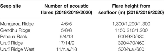
TABLE 1. Overview of seeps observations based on MBES data.

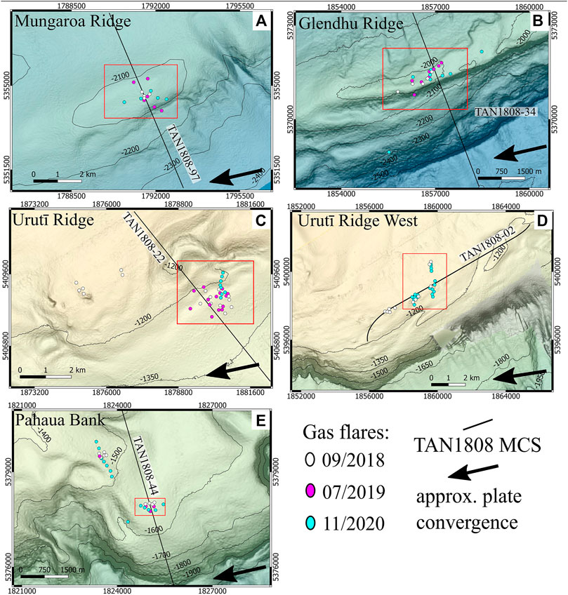
FIGURE 4. Distribution of the gas flares identified in the five target areas: (A) Mungaroa Ridge; (B) Glendhu Ridge; (C) Urutī Ridge; (D) Urutī Ridge West; (E) Pahaua Bank. The approximate direction of plate convergence is extracted from the MORVEL online tool (Argus et al., 2011). MCS, multi-channel seismic data.

Gas Fluxes and Seismic Observations

In this section, we present the results of gas flux estimations for the five target areas (Figure 5) and analyse the local geological structure of these sites.

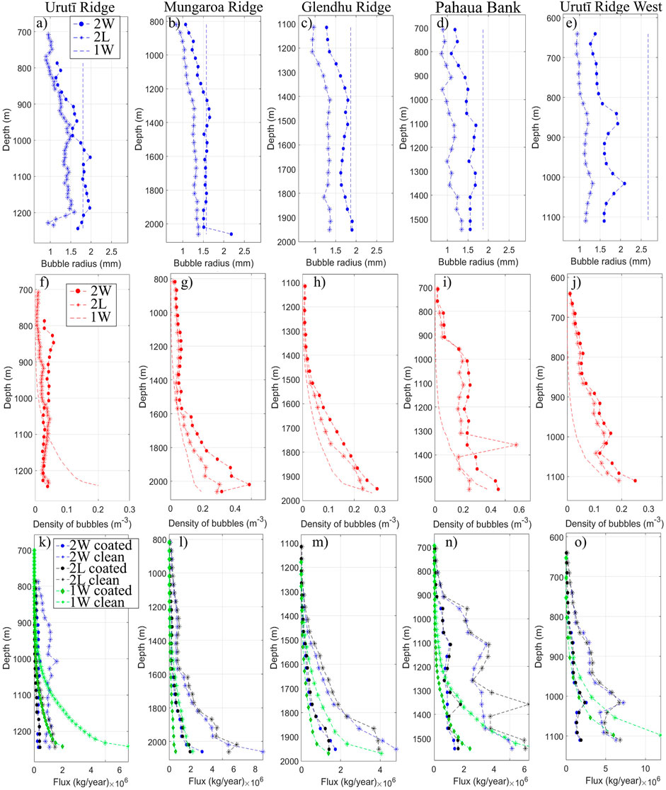
FIGURE 5. Results of methane flux estimations for the five seep locations. (A–E) show the variations of the mean bubble radius versus depth; (F–J) show the mean density of bubbles and (K–O) show the mean methane fluxes calculated at depth with the clean and coated ascending velocity models. 2 W: linear inversion with Weibull distribution; 2 L: linear inversion with log-normal distribution; 1 W: manual curve fitting with Weibull distribution.

At each seep site, we selected one representative flare from the SBES data (shown in Figures 7–10). The selection was driven by data quality, representativeness of the flare for the entire seep field, and vicinity to the location of the seismic line. The selected flares were used to estimate bubble size parameters and bubble density, which were considered to be representative of all the seeps located in the same field.

The flux estimates provided in the following sections represent an average of the linear inversion method (Approach 2), while the comparison of the results of the manual curve fitting (Approach 1) is shown in Figure 5 and in Table 2, together with the details of the parametrization of gas flares for each of the target sites.

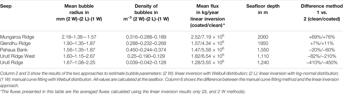
TABLE 2. Details of bubble size parameters, density of bubbles, mean gas fluxes and seep water depth for the five target areas.

The average thickness of the gas hydrate stability zone (GHSZ) varies according to the water depth and the geological context, from ∼360 m at Urutī Ridge (1,200 mbsl) to ∼630 m at Mungaroa Ridge (2,100 mbsl). Despite being visible throughout the five study areas, bottom-simulating reflections (BSR) associated with gas hydrate occurrence are discontinuous and cannot be observed directly below the locations of gas seepage. In Figures 7–11, the vertical and horizontal scales of the EK60 echograms showing the gas flares are approximately equal to the scales of the seismic image. It is important to note that the acoustic images of the water column show the apparent resolution of the EK60 data: the true horizontal resolution depends on the beamwidth and varies with depth following:

Where r is the horizontal resolution, r^∗ is the apparent resolution, d is the water depth and θ is the beam aperture angle (Figure 6). Seismic velocity of 1700 m/s (Turco et al., 2020) was used to depth convert the seismic sections, whereas the echograms were depth-converted on-the-fly during data acquisition using sound velocity profiles. The dominant frequency of the processed seismic data is 95 Hz, and the vertical resolution is approximately 4–5 m. The acquisition and processing parameters of the seismic data are provided by Crutchley et al. (2018) and Turco et al. (2020), respectively.

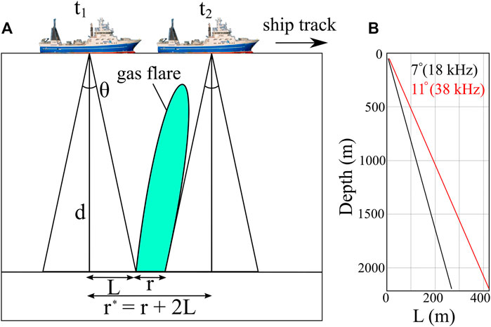
FIGURE 6. (A) Graphical illustration of the lateral resolution of the acoustic images of the single-beam (EK60) data. (B) Plot showing the dependence of the lateral resolution (L) on water depth and beam angle.

Urutī Ridge

The main Urutī Ridge seep field is located slightly seaward of the bathymetric high of the anticlinal ridge. The seepage occurs over ∼4 km² of the seafloor, in water depths from 1,175 m to 1,300 m, and tens of flares can be identified from the acoustic data (17 flares identified in the 2018 datasets, 14 flares in 2019 and 9 in 2020). The same flares were imaged in all surveys. Most acoustic flares reach ∼700 m water depth, and the total area of high acoustic anomaly at 20 m above the seafloor measures 0.43 km². The easternmost flares imaged in the TAN2012 dataset seem to be aligned roughly NS, which is sub-perpendicular to the direction of plate convergence in this part of the margin. The main flare was selected from the total population of flares of this region to estimate the density of bubbles per cubic metre. Gas flux estimates for the entire seep field at Urutī Ridge range between 1.28 and 3.55 × 10⁶ kg/year. The seismic profile shown in Figure 7 runs perpendicular to the strike of the main anticlinal structure, and it crosses the seabed location of two major gas flares used for flux estimations. A broad extent of ∼1 km of the shallow subsurface shows high-amplitude negative polarity reflections that reveal the presence of free gas in the sediments. The sedimentary sequence below this region is characterized by a general decrease in seismic amplitudes (seismic blanking) and disrupted reflections. The blanking zone in the overlying stratigraphic sequence is bounded in depth by a seismic unconformity that marks the top of a highly reflective unit of steeply dipping strata that form the seaward limb of the Urutī Ridge anticline. The amplitude of the BSR is higher to the NW and to the SE of the flare site, it fades out in the core region of the anticline, and it is not observed in the region of enhanced reflectivity on the seaward limb of the anticline.

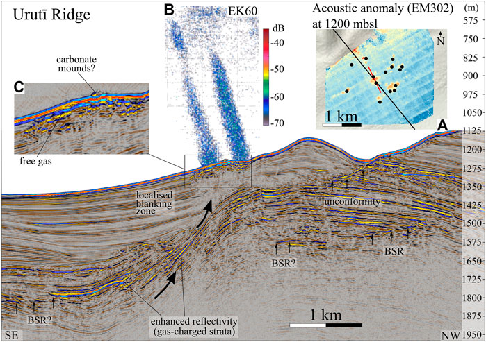
FIGURE 7. Overview of the Urutī Ridge seep site: the interpreted TAN1808-22 seismic profile is shown in the main panel. The bold black arrows represent the direction of fluid flow as interpreted from the seismic data and explained in the text. BSR, bottom simulating reflection. (A) Map view of the Urutī Ridge seeps (red box in Figure 4C), showing the acoustic backscatter anomaly in the echo integrated MBES (EM302) data in proximity of the seafloor. The location of the TAN1808-22 seismic line and of the single-beam data (EK60) are indicated by the black and the red lines, respectively. The black dots represent the location of the main gas flares. The hydroacoustic data were collected during the TAN1904 voyage. (B) Echogram of two gas flares as imaged by the 18 kHz channel in the single-beam data. The horizontal scale is the same as the seismic panel. (C) Expanded view of the seismic data showing the shallow region beneath the cold seeps.

Glendhu Ridge

Glendhu Ridge is a thrust-related elongated structural feature with four-way closure that lies close to the present-day deformation front. The anticlinal structure of the ridge is imaged in the seismic profiles and has been analysed in detail by Turco et al. (2020). There is no BSR below the seep location at the top of the ridge, similar to what is observed at Urutī Ridge (Figure 7). The main gas venting field is located right on the bathymetric crest of the ridge, at a water depth of about 2000 m, where 6–8 main acoustic flares can be identified from the multibeam data. The seeps are roughly aligned ENE-WSW, parallel to the long-axis of the four-way closure and sub-parallel to the vector of plate convergence (Figure 4B). For the parametrization of this gas seep field, we used the main acoustic flare visible in Figure 8, which rises from the seafloor for roughly 1,200 m reaching a depth of ∼780 mbsl. The area of acoustic anomaly at this site is 0.17 km², yielding total gas flux estimates of 1.57 and 4.34 × 10⁶ kg/year, considering coated and clean bubbles, respectively.

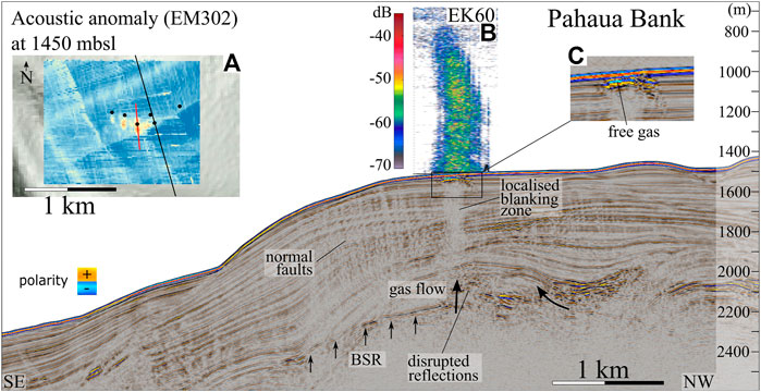
FIGURE 8. Overview of the Pahaua Bank seep site: the interpreted TAN1808-44 seismic profile is shown in the main panel. The bold black arrows represent the direction of fluid flow as interpreted from the seismic data and explained in the text. BSR: bottom simulating reflection. (A) Map view of the Pahaua Bank seeps (red box in Figure 4E), showing the acoustic backscatter anomaly in the echo integrated MBES (EM302) data in proximity of the seafloor. The location of the TAN1808-44 seismic line and of the single-beam data (EK60) are indicated by the black and the red lines, respectively. The black dots show the locations of the main gas flares. The hydroacoustic data were collected during the TAN1904 voyage. (B) Echogram of a gas flare as imaged by the 18 kHz channel in the single-beam data. The horizontal scale is the same as the seismic panel. (C) Expanded view of the seismic data showing the shallow region beneath the cold seeps, where free gas accumulation is inferred by the negative polarity reflection.

Pahaua Bank

Pahaua Bank is a submarine ridge located on the mid-slope portion of the accretionary wedge, at water depths of 1,450–1,570 m. There are two regions of gas seepage at the seafloor: the northernmost group of gas seeps includes at least seven distinct flares aligned NNW-SSE, perpendicular to the direction of plate convergence (Figure 4E). The southernmost group consists of at least six flares rising from 1,560 m. In both groups, the acoustic signature of the rising bubbles reaches the depth of ∼750 mbsl. The total area of acoustic anomaly close to the seafloor measures 0.21 km². One flare from the southernmost group was used for bubble size and density parametrization, yielding gas flux estimates between 1.47 and 5.58 × 10⁶ kg/year for this site. The seismic data reveal a ∼400 m long, strong reflection with negative polarity right below the seabed at the location of gas seepage, indicative of widespread free gas in the shallow sediments (Figure 8C). Below the free gas accumulation, a column-shaped region of localised seismic blanking extends downwards towards the base of the GHSZ, in a region of disrupted reflections in the vicinity of an apparent BSR shoaling.

Urutī Ridge West

This is the shallowest of the analysed seep fields, and it lies in a region of relatively flat bathymetry at ∼1,140 m water depth. Urutī Ridge West is a SW-NE trending anticline that represents the southern extension of Urutī Ridge. The seismic profile shown in Figure 9 runs parallel to the strike of the anticline, and crosses two areas of gas seepage. The sedimentary sequence is characterised by relatively flat and parallel strata. The thickness of the GHSZ at Urutī Ridge West is ∼0.5 s, or ∼450 m using an estimated seismic velocity of 1800 m/s. While the BSR appears as a distinct negative polarity reflection adjacent to the seep locations, it is characterised by a series of lower amplitude reflections in the central part of the seismic profile, and it is not imaged beneath the regions of gas expulsion. High amplitude reflections with the same polarity as the seafloor probably point to the presence of concentrated gas hydrates or authigenic carbonates in the shallow sediments, while column-shaped regions of seismic blanking suggest upward fluid migration from the base of gas hydrate stability (BGHS) towards the seafloor. Similar to the Urutī Ridge eastern flares and to the Pahaua Bank northern flares, the gas flares at Urutī Ridge West are aligned roughly perpendicularly to the direction of plate convergence. The 18 imaged flares can be grouped into four clusters (Figure 4D), and they rise ∼500 m from the seafloor. One flare was selected to estimate bubble parameters (see Table 2). With a total area ∼0.45 km² of acoustic anomaly, the gas flux estimates for the Urutī Ridge West venting field lie between 1.82 and 6.54 × 10⁶ kg/year.

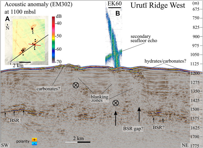
FIGURE 9. Overview of the Urutī Ridge West seep site: the interpreted TAN1808-02 seismic profile is shown in the main panel. The black arrows show the direction of fluid flow as interpreted from the seismic data and explained in the text. The black crossed circles represent the direction of fluid flow going into the page. BSR: bottom simulating reflection. (A) Map view of the Urutī Ridge West seeps (red box in Figure 4D), showing the acoustic backscatter anomaly in the echo integrated MBES (EM302) data in proximity of the seafloor. The location of the TAN 1808-02 seismic line and of the single-beam data (EK60) are indicated by the black and the red lines, respectively. The black dots show the locations of the main gas flares. The hydroacoustic data were collected during the TAN2012 voyage. (B) Echogram of a gas flare as imaged by the 38 kHz channel in the single-beam data. The horizontal scale is the same as the seismic panel.

Mungaroa Ridge

The Mungaroa seep field (Figure 10) is the deepest analysed in this study, with its main gas flare located at 2080 mbsl at the top of Mungaroa Ridge, a thrust-related four-way closure that lies at the toe of the accretionary wedge. Crutchley et al. (2021) investigated the gas hydrate system and fuid flow processes at Mungaroa Ridge in detail, using seismic reflection and multibeam data. They interpreted a gas-water contact pointing to a thick free gas column beneath the BGHS (Figure 10). This gas column is sufficiently thick to cause hydraulic fracturing through the gas hydrate stability zone, which is evidenced by a vertical chimney structure connecting the gas reservoir to the seafloor gas flare. Despite the existence of normal faults beneath the ridge, Crutchley et al. (2021) noted that they are not exploited for focused gas flow into the hydrate stability zone. We surveyed the region of gas seepage at the seafloor of Mungaroa Ridge during the three R/V Tangaroa voyages. From these data, we observed six flares rising from the seabed up to roughly 600 mbsl, making them the highest flares observed in the region (∼1,400 m high). The estimated methane fluxes at this site range from 2.52 to 7.18 × 10⁶ kg/year.

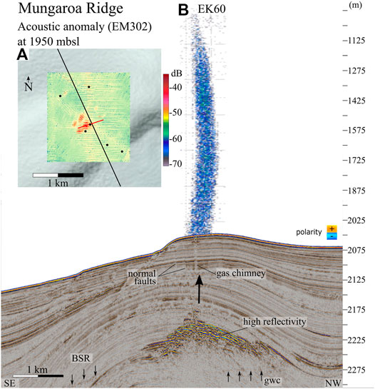
FIGURE 10. Overview of the Mungaroa Ridge seep site: the interpreted TAN 1808-97 seismic profile is shown in the main panel (interpretation after Crutchley et al., 2021). The bold black arrow shows the direction of fluid flow as interpreted from the seismic data and explained in the text. BSR: bottom simulating reflection; gwc: gas-water contact. (A) Map view of the Mungaroa Ridge seeps (red box in Figure 4A), showing the acoustic backscatter anomaly in the echo integrated MBES (EM302) data in proximity of the seafloor. The location of the TAN1808-97 seismic line and of the single-beam data (EK60) are indicated by the black and the red lines, respectively. The black dots represent the locations of the main gas flares. The hydroacoustic data were collected during the TAN2012 voyage. (B) Echogram of a gas flare as imaged by the 38 kHz channel in the single-beam data.

Discussion

The quantitative study of water column acoustic backscatter data combined with observations of subsurface geological structures has allowed a detailed characterisation of the five targeted cold seep areas on the southern Hikurangi Margin.

Sources of Uncertainty for Flux Estimations

There are several sources of uncertainty in the resulting estimations of gas fluxes at the seafloor.

The major source of uncertainty comes from the theoretical model used to predict bubble rising velocities. Because of the lack of quantitative observational data in the study area, we opted for using both clean and coated bubble models (Leifer and Patro, 2002) for our flux estimates.

Another type of uncertainty to be considered is related to instrumental parameters, that account for uncertainties of calibration, sound-velocity profiles and absorption rates. The calculated uncertainty for the SBES absolute backscatter measurements is ∼0.2 dB. The uncertainty of the absolute $S_v$ backscatter data will propagate on through the calculation of both BSD parameters and density of bubbles and will eventually affect flux estimations. However, due to the relatively high precision of the echo-sounders, we deem the effect of instrumental uncertainty negligible compared to the other sources of variability described in this and in the next section.

For the MBES data, usually 1–2% of the water depth is considered a conservative uncertainty in terms of positioning of soundings. Considering the deepest flare at Mungaroa Ridge (2080 mbsl) the highest uncertainty related to the spatial extent of the acoustic anomalies in the MBES data is of ∼1,600 m². This translates in ±2 × 10⁴ and ±3.01 × 10⁵ kg/year of methane considering coated and clean bubble models, respectively.

Uncertainties related to the estimations of bubble parameters, such as mean radius, bubble density and bubble size distribution, are addressed in detail in the next section.

Constraints on Bubble Size Distributions

Quantification of gas flux is dependent on observations of bubble parameters. Ideally, optical measurements such as video observation, bubble size measuring, and sampling of the seep fluids provide the most accurate measures of the bubble size distribution function, their rising velocity, and the chemical gas composition, enabling the determination of realistic values of gas flow rates (e.g., von Deimling et al., 2011; Higgs et al., 2019; Wang et al., 2016; Weber et al., 2014).

Due to the lack of optical observations of the seeps analysed in this study, no measurements of BSD are available, and we adopt a variation of the method proposed by Veloso et al. (2015) to estimate the BSD from the split-beam EK60 data. To test the validity of the results, we analyse the dependence of the estimated methane fluxes on different BSD functions: we first parametrise the BSD by assuming log-normal and Weibull probability density functions (PDF), and then compare the inverted results (Figure 11). The choice of these PDFs was made based on published seep studies, which have suggested several distribution functions to describe bubble size data including normal (Römer et al., 2012), log-normal (Veloso et al., 2015; Wang et al., 2016; Li et al., 2020), and Weibull (Dey and Kundu, 2012).

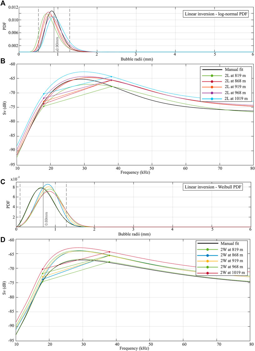
FIGURE 11. Bubble size distributions estimated from linear inversion of the split-beam data at the Mungaroa Ridge gas flare, imposing log-normal (A) and Weibull (C) distributions. Each curve is representative of a 50 m high horizontal slice of the gas flare, and is color coded according to the water depth. (B) and (D) show the theoretical frequency response curves at each horizontal slice of the gas flare, and the dots represent the observed S_v at the same water depth for the 18 and the 38 kHz channels.

The modelled $S_v$ depends on both the BSD and the density of bubbles (e.g., MacLennan et al., 2002). If the BSD parameters are over corrected during the curve matching procedure, the density of bubbles will be underestimated, so that the final impact on the calculation of gas fluxes is minimal. This can be observed, for example, in the inversion results for the Mungaroa Ridge flare at 2060 mbsl (Figure 10), where the mean bubble radius of the BSD modelled assuming a Weibull distribution increases above 2 mm, the density of bubbles for the corresponding depth shows a sharp decrease. The number of bubbles smaller than 0.5 mm is probably overestimated by the Weibull PDF, and the log-normal curves are more likely to represent the real BSD at these seep sites.

The use of two different approaches to estimate bubble parameters allows us to quantify the degree of agreement between the two methods. The fluxes estimated assuming a constant BSD for the entire flare and based on the normalised $S_v$ response (Approach 1–manual curve fitting method) show a general smooth trend with depth (Figures 5K–O). This trend can be explained by the fact that in this approach a mean $\overline{S_v}$ is calculated by averaging the echo integrated backscatter volume strength of the cells located at the same depth. Through this approach, we obtain one mean bubble radius per site rather than a profile of radii changing with depth. Because of the stronger response of bigger bubbles close to the emission site this method will also tend to overestimate the mean of the BSD, as the overall response of the flare is dominated by this area, as observed in Figures 5A–E. Despite this approximation, the manual curve fitting approach is a useful method that can be used to obtain informed starting models for the linear inversion method. Because of its deterministic nature, the second approach (linear inversion) requires the existence of a solid starting model in order to converge to a global minimum. This method provides a more reliable tool to track changes of physical parameters of the bubbles in the water column. The fluxes calculated through the linear inversion method (both assuming Weibull and log-normal distributions) show more variability in the calculated density of bubbles and fluxes, despite a general increase with depth (e.g., Figure 5). Table 2 summarizes the differences in the results of the two approaches. The differences between flux estimates calculated using a constant BSD for the entire flare (approach 1) and the fluxes obtained through the linear inversion process (approach 2) can be over 400%. For these reasons, we deem the flux estimates calculated through linear inversion more reliable (Table 2), and use those to extrapolate margin-wide flux estimates.

Source of Gas and Seismic Manifestation of Fluid Flow

The southern Hikurangi Margin is a well-established province of gas hydrate occurrence, focussed fluid migration and gas seepage (e.g., Barnes et al., 2010; Crutchley et al., 2019; Kroeger et al., 2019; Watson et al., 2020). Consistent with most subduction margins, the analysis of gases emitted at the seafloor suggests a predominantly microbial origin of methane over a thermogenic origin (Greinert et al., 2001; Faure et al., 2010). The co-location of high-resolution seismic reflection images and water column imaging (EK60 data) enables us to compare the sub-seafloor with the water column at gas seep locations.

At all the flare sites observed in this study, we found evidence of gas migrating from beneath the base of the GHSZ to the seafloor. In the case of Mungaroa Ridge, a large free gas reservoir in the core region of the anticline has been interpreted by Crutchley et al. (2021) as the source that supplies gas to the main seep observed at the seafloor. Here, Crutchley et al. (2021) suggest that over-pressured gas causes hydraulic fracturing of the overlying sediments leading to the formation of the vertical gas chimney imaged in the seismic data (Figure 10). The presence of such large and interconnected free gas accumulations is not observed at the other target sites of this study. However, highly reflective strata are imaged directly beneath the base of the GHSZ at Urutī and Glendhu ridges, as well as at Pahauau Bank. The enhanced reflectivity is likely to be caused by the strong impedance contrast between fine-grained low-permeability layers and sandy gas-charged sedimentary units, as interpreted by Turco et al. (2020) at Glendhu Ridge. Stratigraphically driven fluid migration along permeable dipping strata has been suggested to be the main mechanism for upward fluid flow in many anticline-related ridges on the Hikurangi Margin (e.g., Crutchley et al., 2019; Wang et al., 2017a; Turco et al., 2020; Barnes et al., 2010; Kroeger et al., 2021). Urutī Ridge is a good example of this process, where highly reflective strata appear to be transporting gas from depth upward into the GHSZ (Figure 6). At Urutī Ridge, Urutī Ridge West, Pahaua Bank ,and Glendhu Ridge, fluid migration through the GHSZ is also identified by areas of decreased amplitude (seismic blanking) and disrupted stratigraphic reflections beneath the seeps (Figures 6–9). Seismic blanking is often caused by strong signal attenuation at the seafloor or within the shallow sub-seafloor, caused by the presence of highly reflective interfaces. Such interfaces could come from authigenic carbonates or gas hydrate accumulations (e.g., Bohrmann et al., 1998). The disruption of reflections can be due to the scattering of seismic energy caused by the presence of gas (Judd and Hovland, 1992) or by physical disruption of layering caused by focused gas migration (e.g., Davis 1992; Gorman et al., 2002). While free-gas occurrence is likely to cause most of the seismic blanking observed beneath the seep sites, the presence of autigenic carbonates on the seafloor might contribute to the loss of seismic energy transmission in high-frequency data. In summary, the seismic images show a diversity of manifestations of free gas in the sub-seafloor, ranging from gas-water contacts at the base of a free gas reservoir (Mungaroa Ridge; Figure 10) through layer-parallel gas migration (e.g., Urutī Ridge; Figure 6) to vertical gas migration facilitated by hydraulic fracturing (Flemings et al., 2003; e.g., Pahaua Bank and Mungaroa Ridge; Figures 8, 10).

Temporal Variability of the Seeps

There are many mechanisms that control the activity of different types of gas seeps. Consequently, the time scales over which the activity of cold seeps fluctuates can span from minutes to millennia. For example, Feseker et al. (2014) document the eruption of a deep-sea mud volcano that triggered large methane and CO₂ emissions over a period of minutes. Pressure changes at the seafloor caused by tides have been shown to impact the flow rate of shallow and deep-sea gas seeps (Boles et al., 2001; Römer et al., 2016; Riedel et al., 2018), while seasonal sea-bottom temperature variations can cause cold seeps to hibernate during the cold months, trapping gas in the sediments that is released in pulses during warmer months (Berndt et al., 2014; Ferré et al., 2020). On the other hand, natural seismicity (Franek et al., 2017) and ocean warming (Baumberger et al., 2018) are potential triggers for significant release of methane from the sediments, especially in hydrate provinces.

Our study represents an opportunity to analyse the variability of methane emissions on the southern Hikurangi Margin over a three-year period. Although quantitative estimates were calculated only once for each gas flare, from either the 2019 or from the 2020 datasets, from the qualitative analysis of multibeam and split-beam data, no substantial difference could be observed in the activity of the main seeps at the time of each survey (Figure 12). In fact, the spatial extent of the acoustic anomaly close to the seafloor remains constant for the five target areas in the three datasets, as does the height of the acoustic flares.

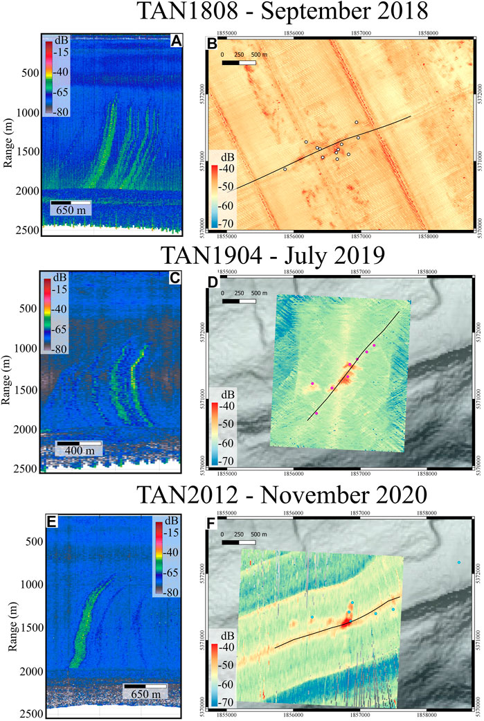
FIGURE 12. Evolution of the Glendhu Ridge seep site over the years. The panels on the left (A,C,E) show range stacked views of MBES (EM302) data of the gas flares on the top of Glendhu Ridge from TAN1808, TAN1904, and TAN2012 datasets, respectively. The panels on the right (B,D,F) show the acoustic backscatter anomaly in the echo integrated MBES data in proximity of the seafloor. The black lines represent the ship track shown in the left panels. The coordinate system is UTM Zone 60 S (WGS84 datum).

In addition to acoustic observations, it is known from authigenic carbonates (for example on Urutī Ridge) that many of the seep sites have been active for thousands of years (e.g., Jones et al., 2010; Liebetrau et al., 2010). Likewise, there is evidence for stable methane seepage over intermediate timescales from tube worms (Lamellibrachia spp.) up to 2 m long sampled at Mungaroa, Urutī and Glendhu ridges (TAN1904 Voyage Report, NIWA). Tube worms of this species require at least 200 years to reach such lengths (Fisher et al., 1997; Cordes et al., 2007).

While the combination of acoustic observation and bio-geological sampling might indicate a constant seepage activity throughout this time, we cannot rule out that methane fluxes vary over seasonal or shorter cycles. For simplitity, we assume a constant discharge rate for the flux estimates presented in this work. Understanding and monitoring the temporal variability of a field of cold seeps is relevant to several scientific and socio-economic issues. At a national scale, one of the most direct implications is related to regional ecosystem management. Cold seeps are increasingly recognized as centres of local biogeochemical cycling and oases for many animals with recent studies finding that commercially important fisheries species are associated with seep habitats and consume methane derived carbon from chemosynthetic production in seep systems (Grupe et al., 2015; Levin et al., 2016; Seabrook et al., 2019; Turner et al., 2019).

Margin-Wide Estimates of Seafloor Methane Flux

To refine our understanding of the global carbon budget, it is important to study the potential implications of seabed gas release on a regional scale. To this end, the relevance of margin-wide studies on natural methane seeps has increased in the past decade: Pohlman et al. (2011) found that up to 28% of the total dissolved organic carbon derives from fossil methane, while Garcia-Tigreros et al. (2021) conclude that aerobic oxidation of CH₄ has a greater influence on ocean chemistry in regions where methane concentrations are locally elevated. Based on the analysis of more than 300 gas seeps, Riedel et al. (2018) estimate a combined average in-situ flow rate of about 88 × 10⁶ kg/year for the Cascadia Margin. Sahling et al. (2014) calculate the gas flux on the western margin of Svalbard to be between 0.11 and 1.89 × 10⁶ kg/year, while the combined methane leakage from the seafloor on the US Atlantic Margin is estimated to range between 1.5 and 90 × 10⁴ kg/year (Skarke et al., 2014). About 0.13–1.01 × 10⁶ kg of methane per year have been estimated to leak from gas seep fields on the Makran Margin offshore Pakistan (Römer et al., 2012).

The distribution of gas seeps on the Hikurangi Margin has been investigated in detail by Watson et al. (2020), who identified 1,457 gas flares from water column data, spanning from East Cape to Kekerengu Bank, off Kaikōura peninsula, in an area of approximately 51,215 km² (Figure 2A). If we consider the flux estimates presented in this paper for the five analyzed seep fields, and we divide them by the number of flares observed at each site, we obtain average methane fluxes per flare between 1.9 × 10⁵ and 6.4 × 10⁵ kg/year, considering coated bubbles and clean bubbles models, respectively. Multiplying by the number of observed flares from Watson et al. (2020), we can extrapolate a total flux ranging between 2.77 × 10⁸ and 9.32 × 10⁸ kg of methane released each year on the whole Hikurangi Margin. These estimates correspond to, respectively, ∼67 and ∼233% of the total amount of methane that was released in 2019 from land sources in New Zealand (i.e., 4.121 × 10⁸ kg/year New Zealand Ministry for Environment—Manatū Mō Te Taiao, www.environment.govt.nz). It is worth pointing out that these estimates might represent an underestimation of the real methane flux occurring on the margin, because they are based solely on acoustic evidence of focused fluid flow (i.e., gas bubbles in the water), and do not take into account diffusive fluid seepage, which is also inferred to occur on the Hikurangi Margin (Watson et al., 2020). On the other hand, assuming a constant methane discharge at the seep sites over seasonal or shorter cycles might lead to an overestimation of annual gas fluxes. Similarly, the assumption that all flares in the same seep field have identical bubble parameters is an approximation that can result in overestimating methane discharge at smaller seeps. To better assess the methane fluxes, long term observational data and chemical sampling at the analysed sites might be required.

Potential Implications for Ocean pH and Local Deoxygenation

From the acoustic imaging of the water column, no evidence was found that methane bubbles reach the sea surface at any of the analysed flares. Considering the depth of the seep sites reported here, two different processes will interact to prevent the CH₄ emitted at the seafloor from reaching the atmosphere: 1) the methane contained in the bubbles will dissolve into the water driven by the low concentration of CH₄ in the ocean (Wiesenburg and Guinasso, 1979), and2) dissolved CH₄ is converted into CO₂ in the water column by abiotic and biotic forces (McGinnis et al., 2006). Although bubble-stripping and methane oxidation reduce the amount of CH₄ released into the atmosphere, these processes can significantly impact local marine habitats and ocean chemistry.

As the majority of the CH₄ emitted by cold seeps remains in deep waters, aerobic oxidation is a primary sink for the methane, as well as a source of CO₂. This CO₂ production needs to be considered with respect to acidification of deep water (Archer et al., 2009; Biastoch et al., 2011), particularly as seeps represent a more direct source in deep water than the transfer of anthropogenic carbon via deep water formation and transport. Large-scale methane release has resulted in ocean acidification in earths geological past (Zachos et al., 2005), but assessments of the current contribution of methane seeps indicate a relatively minor impact on deep water pH (Garcia-Tigreros and Kessler, 2018). However, this source may become significant in response to warming and associated destabilisation of methane hydrates in regions such as the Arctic (Biastoch et al., 2011).

In the current study we estimated the regional contribution to deep waters on the Hikurangi Margin by scaling up the methane release estimated from the bubble plumes to the total number of flares identified in the acoustic data (Watson et al., 2020). Assuming this methane loading was uniformly distributed within the bottom 100 m of water overlying the sediment for the entire margin, from East Cape to the Kaikoura peninsula, provided an estimate of total input of 2.77 × 10⁸ and 9.32 × 108 kg methane/year, based upon the clean and coated bubbles models, respectively. If 100% of this methane is oxidised to CO₂ then the resulting change in the carbonate system, calculated using measured bottom water dissolved inorganic carbon, total alkalinity, temperature, and salinity (C. Law, pers. comm.) in the CO₂sys programme (Hunter, 2015), would result in a decrease in pH_T of 0.048–0.144 relative to the background value of 7.962. These estimates are conservative, and suggest a relatively minor impact to a significant decrease in regional pH, with the upper estimate exceeding the surface ocean pH decrease arising from anthropogenic CO₂ emissions to date (Orr et al., 2005), and comparable to 50% of the projected pH decrease in New Zealand waters by the end of this century (Law et al., 2018). A reduction in pH of this magnitude could have significant impacts on benthic calcifying organisms, particularly as the Hikurangi Margin gas seeps are within the regional depth range of the Aragonite Saturation Horizon (Bostock et al., 2015), below which solid carbonate becomes thermodynamically unstable. However, this estimate of pH decrease should be regarded as an upper limit, as dilution and transport of methane in and out of the region are not considered in this estimate. Refined estimates of pH change require direct measurement of dissolved methane and regional modelling of methane distribution and dispersion using ROMS (Hadfield et al., 2007).

The aerobic oxidation of methane (methanotrophy) by free-living and symbiont-associated bacteria occurs in the seafloor and water column around sites of gas release (Steinle et al., 2015; Sweetman et al., 2017; Levin, 2018). Although not analysed in this study, the aerobic oxidation of methane to CO₂ can also cause localized deoxygenation at a regional scale, impacting ecosystem health and species distribution (Boetius and Wenzhöfer, 2013; Breitburg et al., 2018). Throughout the global ocean there has been an oxygen loss of at least 2% over the past 50–100 years, with well understood linkages of ocean warming reducing oxygen solubility and ocean ventilation (Dickens, 2001; Levin, 2018). However, the influence of features that influence dissolve oxygen at regional scales, such as methane seeps, remains unclear. In addition to the direct effect of methanotrophy, some evidence suggests that seeps with strong bubble plumes, such as observed at some of sites reported here, can draw nutrient and hydrocarbon rich water towards the surface, stimulating primary production and eventually drawing down oxygen as well (Levin, 2018). The potential scale of this process could be significant, as seen in the aftermath of the Deepwater Horizon oil spill in the Gulf of Mexico, where a major reduction of oxygen was measured ad microbial communities released from the spill (Kessler et al., 2011). The downstream ecological and biogeochemical impacts of the release of large volumes of methane by the Hikurangi Margin seeps, as detailed in this study, warrants further scientific attention to understand the implications of future change.

Conclusion

The combination of seismic and hydroacoustic data analysis allowed the characterisation of five cold seep sites on the southern Hikurangi Margin in terms of geological setting and gas flux estimates. Seismic imaging of the geological structures underlying the seep sitesprovided insights into the origin of the gas in the subsurface. Hydroacoustic data collected over 3 years allowed mapping of the backscatter anomalies near the seafloor at the sites of seepage and pinpointing the location of the main gas flares on the seabed. A total of 43, 33, and 53 individual flares were identified from the TAN1808, TAN1904, and TAN2012 datasets, respectively.

The use of the multi-frequency split-beam echosounder allowed estimates of the gas flux rates at the five target sites to be made. The five cold seep fields analysed in this study on the southern Hikurangi Margin of New Zealand lie in water depths ranging from 1,110 to 2060 m, and emit, combined, between 8.66 and 27. 21 × 10⁶ kg of gas per year. The extrapolated methane flux for the whole Hikurangi Margin range between 2.77 × 10⁸ and 9.32 × 10⁸ kg of methane released each year. These estimates are based on acoustic evidence of focused fluid flow, and do not take into account diffusive seafloor seepage.

The results of this study provide the most quantitative assessment to date of total methane release on the Hikurangi Margin, filling gaps of unknown methane sources and better constraining models of ocean acidification and deoxygenation. Moreover, the fluxes presented here can be used as a proxy to monitor changes in the flux rates over the mid-to long term associated with ocean warming.

Data Availability Statement

The raw data supporting the conclusions of this article will be made available by the authors, without undue reservation.

Author Contributions

FT: conceptualization, literature review, acoustic, and seismic data acquisition (TAN1808–TAN2012), acoustic data processing, software developing for flux estimates, writing. YL: gas bubble project leader, supervision in the methodology, software developing for acoustic data analysis, and processing, data curation. SW: gas bubble project leader, writing–review, supervision, seismic, and acoustic data acquisition (TAN1808). CL: took care of the ocean acidification implications and estimates on pH change, writing–review. GJC: gas hydrate seismic project leader, conceptualization of manuscript, especially discussion, seismic and acoustic data acquisition and processing (TAN1808), writing–review. SS: contribution to writing biogeochemical implication of the study, acoustic data acquisition (TAN1904). JM: supervision, seismic and acoustic data acquisition (TAN1808), supervision, project management and facilities. CL: contribution to calculating CO₂ for ocean acidification, acquisition of acoustic data (TAN1904). IP: gas bubble project co-leader, acoustic data acquisition (TAN2012), writing–review. JITH: gas hydrate project leader, seismic and acoustic data acquisition (TAN1808), writing–review. SW: seismic data acquisition and processing (TAN1808), acoustic data acquisition (TAN2012). AG: supervision, provided facilities and funding.

Funding

Part of this work has been carried out within the HYDEE research programme, funded by the New Zealand’s Ministry for Business, Innovation and Employment, contract no. C05X1708, and is included a Ph.D. thesis from the University of Otago (Turco, 2021). Part of the funding came from the Smart Idea project Broadband acoustic characterization of free gases in the ocean water, contract nr. C01X1915.

Conflict of Interest

The authors declare that the research was conducted in the absence of any commercial or financial relationships that could be construed as a potential conflict of interest.

Publisher’s Note

All claims expressed in this article are solely those of the authors and do not necessarily represent those of their affiliated organizations, or those of the publisher, the editors, and the reviewers. Any product that may be evaluated in this article, or claim that may be made by its manufacturer, is not guaranteed or endorsed by the publisher.

References

Ainslie, M. A., and Leighton, T. G. (2009). Near Resonant Bubble Acoustic Cross-Section Corrections, Including Examples from Oceanography, Volcanology, and Biomedical Ultrasound. J. Acoust. Soc. Am. 126 (5), 2163–2175. doi:10.1121/1.3180130
Archer, D., Buffett, B., and Brovkin, V. (2009). Ocean Methane Hydrates as a Slow Tipping point in the Global Carbon Cycle. Proc. Natl. Acad. Sci. U S A. 106 (49), 20596–20601. doi:10.1073/pnas.0800885105
Argus, D. F., Gordon, R. G., and DeMets, C. (2011). Geologically Current Motion of 56 Plates Relative to the No-Net-Rotation Reference Frame. Geochem. Geophys. Geosystems 12 (11).
Barnes, P. M., Lamarche, G., Bialas, J., Henrys, S., Pecher, I., Netzeband, G. L., et al. (2010). Tectonic and Geological Framework for Gas Hydrates and Cold Seeps on the Hikurangi Subduction Margin, New Zealand. Mar. Geology. 272 (1-4), 26–48. doi:10.1016/j.margeo.2009.03.012
Bassett, D., Sutherland, R., and Henrys, S. (2014). Slow Wavespeeds and Fluid Overpressure in a Region of Shallow Geodetic Locking and Slow Slip, Hikurangi Subduction Margin, New Zealand. Earth Planet. Sci. Lett. 389, 1–13. doi:10.1016/j.epsl.2013.12.021
Baumberger, T., Embley, R. W., Merle, S. G., Lilley, M. D., Raineault, N. A., and Lupton, J. E. (2018). Mantle-derived Helium and Multiple Methane Sources in Gas Bubbles of Cold Seeps along the Cascadia Continental Margin. Geochemistry, Geophysics. Geosystems 19 (11), 4476–4486. doi:10.1029/2018gc007859
Bayrakci, G., Scalabrin, C., Dupré, S., Leblond, I., Tary, J.-B., Lanteri, N., et al. (2014). Acoustic Monitoring of Gas Emissions from the Sea_oor. Part II: a Case Study from the Sea of Marmara. Mar. Geophys. Res. 35 (3), 211–229. doi:10.1007/s11001-014-9227-7
Berndt, C., Feseker, T., Treude, T., Krastel, S., Liebetrau, V., Niemann, H., et al. (2014). Temporal Constraints on Hydrate-Controlled Methane Seepage off Svalbard. Science 343 (6168), 284–287. doi:10.1126/science.1246298
Biastoch, A., Treude, T., Rüpke, L. H., Riebesell, U., Roth, C., Burwicz, E. B., et al. (2011). Rising Arctic Ocean Temperatures Cause Gas Hydrate Destabilization and Ocean Acidi_cation. Geophys. Res. Lett. 38 (8). doi:10.1029/2011GL047222
Boetius, A., and Wenzhöfer, F. (2013). Seafloor Oxygen Consumption Fuelled by Methane from Cold Seeps. Nat. Geosci 6 (9), 725–734. doi:10.1038/ngeo1926
Bohrmann, G., Greinert, J., Suess, E., and Torres, M. (1998). Authigenic Carbonates from the Cascadia Subduction Zone and Their Relation to Gas Hydrate Stability. Geol 26 (7), 647–650. doi:10.1130/0091-7613(1998)026<0647:acftcs>2.3.co;2
Boles, J., Clark, J., Leifer, I., and Washburn, L. (2001). Temporal Variation in Natural Methane Seep Rate Due to Tides, Coal Oil Point Area, California. J. Geophys. Res. Oceans 106 (C11), 27077–27086. doi:10.1029/2000jc000774
Bonini, M. (2019). Seismic Loading of Fault-Controlled Fluid Seepage Systems by Great Subduction Earthquakes. Sci. Rep. 9 (1), 11332. doi:10.1038/s41598-019-47686-4
Bostock, H. C., Tracey, D. M., Currie, K. I., Dunbar, G. B., Handler, M. R., Mikaloff Fletcher, S. E., et al. (2015). The Carbonate Mineralogy and Distribution of Habitat-Forming Deep-Sea Corals in the Southwest pacific Region. Deep Sea Res. Oceanographic Res. Pap. 100, 88–104. doi:10.1016/j.dsr.2015.02.008
Böttner, C., Haeckel, M., Schmidt, M., Berndt, C., Vielstädte, L., Kutsch, J. A., et al. (2020). Greenhouse Gas Emissions from marine Decommissioned Hydrocarbon wells: Leakage Detection, Monitoring and Mitigation Strategies. Int. J. Greenhouse Gas Control. 100, 103119. doi:10.1016/j.ijggc.2020.103119
Breitburg, D., Levin, L. A., Oschlies, A., Grégoire, M., Chavez, F. P., Conley, D. J., et al. (2018). Declining Oxygen in the Global Ocean and Coastal Waters. Science 359 (6371). doi:10.1126/science.aam7240
Colbo, K., Ross, T., Brown, C., and Weber, T. (2014). A Review of Oceanographic Applications of Water Column Data from Multibeam Echosounders. Estuarine, coastal shelf Sci. 145, 41–56. doi:10.1016/j.ecss.2014.04.002
Cook, A. E., and Malinverno, A. (2013). Short Migration of Methane into a Gas Hydrate Bearing Sand Layer at Walker Ridge, Gulf of Mexico. Geochemistry, Geophysics. Geosystems 14 (2), 283–291. doi:10.1002/ggge.20040
Cordes, E. E., Bergquist, D. C., Redding, M. L., and Fisher, C. R. (2007). Patterns of Growth in Cold-Seep Vestimenferans Including Seepiophila Jonesi: a Second Species of Long-Lived Tubeworm. Mar. Ecol. 28 (1), 160–168. doi:10.1111/j.1439-0485.2006.00112.x
Crutchley, G., Fraser, D., Pecher, I., Gorman, A., Maslen, G., and Henrys, S. (2015). Gas Migration into Gas Hydrate-Bearing Sediments on the Southern Hikurangi Margin of New Zealand. J. Geophys. Res. Solid Earth 120 (2), 725–743. doi:10.1002/2014jb011503
Crutchley, G. J., Kroeger, K. F., Pecher, I. A., Gorman, A. R., and Watson, S. (2019). How Tectonic Folding Influences Gas Hydrate Formation: New Zealand’s Hikurangi Subduction Margin. Geology 47 (1), 39–42.
Crutchley, G. J., Mountjoy, J., Hillman, J., Turco, F., Watson, S., Flemings, P., et al. (2021). Upward-doming Zones of Gas Hydrate and Free Gas at the Bases of Gas Chimneys, New Zealand's Hikurangi Margin. J. Geophys. Res. Solid Earth, e2020JB021489. doi:10.1029/2020jb021489
Crutchley, G. J., Mountjoy, J. J., Davy, B. D., Hillman, J. I. T., Watson, S., Stewart, L., et al. (2018). Gas Hydrate Systems of the Southern Hikurangi Margin, Aotearoa, New Zealand. TAN1808 Voyage Report, RV Tangaroa 8-Sep – 5 Oct 2018. Lower Hutt (Nz) GNS Sci., 83p. Avaialble at: https://doi-org.ezproxy.otago.ac.nz/10.21420/73WW-1W83.
Davis, A. M. (1992). Shallow Gas: an Overview. Continental Shelf Res. 12 (10), 1077–1079. doi:10.1016/0278-4343(92)90069-v
De Robertis, A., and Higginbottom, I. (2007). A post-processing Technique to Estimate the Signal-To-Noise Ratio and Remove Echosounder Background Noise. ICES J. Mar. Sci. 64 (6), 1282–1291. doi:10.1093/icesjms/fsm112
Demer, D. A., Berger, L., Bernasconi, M., Bethke, E., Boswell, K., Chu, D., et al. (2015). Calibration of Acoustic Instruments.
Dey, A. K., and Kundu, D. (2012). Discriminating between the Weibull and Log-normal Distributions for Type-II Censored Data. Statistics 46 (2), 197–214. doi:10.1080/02331888.2010.504990
Dickens, G. (2001). On the Fate of Past Gas: What Happens to Methane Released from a Bacterially Mediated Gas Hydrate Capacitor? Geochem. Geophys. Geosystems 2 (1). doi:10.1029/2000gc000131
Duarte, H., Pinheiro, L. M., Teixeira, F. C., and Monteiro, J. H. (2007). High-resolution seismic imaging of gas accumulations and seepage in the sediments of the Ria de Aveiro barrier lagoon (Portugal). Geo-Marine Lett. 27 (2), 115–126. doi:10.1007/s00367-007-0069-z
Dupré, S., Scalabrin, C., Grall, C., Augustin, J.-M., Henry, P., engör, A. C., et al. (2015). Tectonic and Sedimentary Controls on Widespread Gas Emissions in the Sea of Marmara: Results from Systematic, Shipborne Multibeam echo Sounder Water Column Imaging. J. Geophys. Res. Solid Earth 120 (5), 2891–2912. doi:10.1002/2014jb011617
Faure, K., Greinert, J., von Deimling, J. S., McGinnis, D. F., Kipfer, R., et al. (2010). Methane Seepage along the Hikurangi Margin of New Zealand: Geochemical and Physical Data from the Water Column, Sea Surface and Atmosphere. Mar. Geology. 272 (1-4), 170–188. doi:10.1016/j.margeo.2010.01.001
Ferré, B., Jansson, P. G., Moser, M., Serov, P., Portnov, A., Graves, C. A., et al. (2020). Reduced Methane Seepage from Arctic Sediments during Cold Bottom-Water Conditions. Nat. Geosci. 13 (2), 144–148. doi:10.1038/s41561-019-0515-3
Feseker, T., Boetius, A., Wenzhöfer, F., Blandin, J., Olu, K., Yoeger, D., et al. (2014). Eruption of a Deep-Sea Mud Volcano Triggers Rapid Sediment Movement. Nat. Commun. 5 (1). doi:10.1038/ncomms6385
Fisher, C., Urcuyo, I., Simpkins, M., and Nix, E. (1997). Life in the Slow Lane: Growth and Longevity of Cold-Seep Vestimentiferans. Mar. Ecol. 18 (1), 83–94. doi:10.1111/j.1439-0485.1997.tb00428.x
Flemings, P. B., Liu, X., and Winters, W. J. (2003). Critical Pressure and Multiphase Flow in Blake Ridge Gas Hydrates. Geol 31 (12), 1057–1060. doi:10.1130/g19863.1
Franek, P., Plaza-Faverola, A., Mienert, J., Buenz, S., Ferré, B., and Hubbard, A. (2017). Microseismicity Linked to Gas Migration and Leakage on the Western Svalbard Shelf. Geochemistry, Geophysics. Geosystems 18 (12), 4623–4645. doi:10.1002/2017gc007107
Fu, X., Waite, W. F., and Ruppel, C. D. (2020). Hydrate Formation on Marine Seep Bubbles and the Implications for Water Column Methane Dissolution. AGU Fall Meet. Abstr. Vol. 2020, OS016–0006. doi:10.1029/2021jc017363
Garcia-Tigreros, F., and Kessler, J. D. (2018). Limited Acute Influence of Aerobic Methane Oxidation on Ocean Carbon Dioxide and pH in Hudson Canyon, Northern US Atlantic Margin. J. Geophys. Res. Biogeosciences 123 (7), 2135–2144. doi:10.1029/2018jg004384
Garcia-Tigreros, F., Leonte, M., Ruppel, C. D., Ruiz-Angulo, A., Joung, D. J., Young, B., et al. (2021). Estimating the Impact of Seep Methane Oxidation on Ocean pH and Dissolved Inorganic Radiocarbon along the US Mid-Atlantic Bight. J. Geophys. Res. Biogeosciences 126 (1), e2019JG005621. doi:10.1029/2019jg005621
Gorman, A. R., Holbrook, W. S., Hornbach, M. J., Hackwith, K. L., Lizarralde, D., and Pecher, I. (2002). Migration of Methane Gas through the Hydrate Stability Zone in a Low-Flux Hydrate Province. Geol 30 (4), 327–330. doi:10.1130/0091-7613(2002)030<0327:momgtt>2.0.co;2
Greinert, J., Bohrmann, G., and Suess, E. (2001). Gas Hydrate-Associated Carbonates and Methane-Venting at Hydrate Ridge: Classi_cation, Distribution and Origin of Authigenic Lithologies. Geophys. Monograph-American Geophys. Union 124, 99–114. doi:10.1029/gm124p0099
Grupe, B. M., Krach, M. L., Pasulka, A. L., Maloney, J. M., Levin, L. A., and Frieder, C. A. (2015). Methane Seep Ecosystem Functions and Services from a Recently Discovered Southern California Seep. Mar. Ecol. 36, 91–108. doi:10.1111/maec.12243
Hadfield, M. G., Rickard, G. J., and Uddstrom, M. J. (2007). A Hydrodynamic Model of Chatham Rise, New Zealand. New Zealand J. Mar. Freshw. Res. 41 (2), 239–264. doi:10.1080/00288330709509912
Higgs, B., Mountjoy, J., Crutchley, G. J., Townend, J., Ladroit, Y., Greinert, J., et al. (2019). Seep-bubble Characteristics and Gas _ow Rates from a Shallow-Water, High-Density Seep _eld on the Shelf-To-Slope Transition of the Hikurangi Subduction Margin. Mar. Geology. 417, 105985. doi:10.1016/j.margeo.2019.105985
Hillman, J. I., Cook, A. E., Daigle, H., Nole, M., Malinverno, A., Meazell, K., et al. (2017). Gas Hydrate Reservoirs and Gas Migration Mechanisms in the Terrebonne Basin, Gulf of Mexico. Mar. Pet. Geology. 86, 1357–1373. doi:10.1016/j.marpetgeo.2017.07.029
Hillman, J. I., Crutchley, G. J., and Kroeger, K. F. (2020). Investigating the Role of Faults in Fluid Migration and Gas Hydrate Formation along the Southern Hikurangi Margin, New Zealand. Mar. Geophys. Res. 41 (1), 1–19. doi:10.1007/s11001-020-09400-2
Hoffmann, J. J., Gorman, A. R., and Crutchley, G. J. (2019). Seismic Evidence for Repeated Vertical Fluid Flow through Polygonally Faulted Strata in the Canterbury Basin, New Zealand. Mar. Pet. Geology. 109, 317–329. doi:10.1016/j.marpetgeo.2019.06.025
Hornafius, J. S., Quigley, D., and Luyendyk, B. P. (1999). The World's Most Spectacular marine Hydrocarbon Seeps (Coal Oil Point, Santa Barbara Channel, California): Quanti_cation of Emissions. Journal of Geophysical Research:. Oceans 104 (C9), 20703–20711. doi:10.1029/1999jc900148
Hunter, K. (2007). A.: XLCO2 – Seawater CO2 Equilibrium Calculations Using Excel Version 2New Zealand. Dunedin: University of Otago. available at http://neon.otago.ac.nz/research/mfc/people/keith_hunter/software/swco2/(last access February 24, 2015).
Jones, A. T., Greinert, J., Bowden, D., Klaucke, I., Petersen, C. J., Netzeband, G., et al. (2010). Acoustic and Visual Characterisation of Methane-Rich Seabed Seeps at Omakere Ridge on the Hikurangi Margin, New Zealand. Mar. Geology. 272 (1-4), 154–169. doi:10.1016/j.margeo.2009.03.008
Judd, A. G. (2004). Natural Seabed Gas Seeps as Sources of Atmospheric Methane. Environ. Geology. 46 (8), 988–996. doi:10.1007/s00254-004-1083-3
Judd, A., and Hovland, M. (2009). Seabed Fluid Flow: The Impact on Geology, Biology and the marine Environment. Cambridge University Press.
Judd, A., and Hovland, M. (1992). The Evidence of Shallow Gas in marine Sediments. Continental Shelf Res. 12 (10), 1081–1095. doi:10.1016/0278-4343(92)90070-z
Kessler, J. D., Valentine, D. L., Redmond, M. C., Du, M., Chan, E. W., Mendes, S. D., et al. (2011). A Persistent Oxygen Anomaly Reveals the Fate of Spilled Methane in the Deep Gulf of Mexico. Science 331 (6015), 312–315. doi:10.1126/science.1199697
Kim, Y.-J., Cheong, S., Chun, J.-H., Cukur, D., Kim, S.-P., Kim, J.-K., et al. (2020). Identification of Shallow Gas by Seismic Data and AVO Processing: Example from the Southwestern continental Shelf of the Ulleung Basin, East Sea, Korea. Mar. Pet. Geology. 117, 104346. doi:10.1016/j.marpetgeo.2020.104346
Krabbenhoeft, A., Bialas, J., Klaucke, I., Crutchley, G., Papenberg, C., and Netzeband, G. L. (2013). Patterns of Subsurface Fluid Flow at Cold Seeps: The Hikurangi Margin, O_shore New Zealand. Mar. Pet. Geology. 39 (1), 59–73. doi:10.1016/j.marpetgeo.2012.09.008
Kroeger, K., Crutchley, G. J., Kellett, R., and Barnes, P. (2019). A 3-D Model of Gas Generation, Migration, and Gas Hydrate Formation at a Young Convergent Margin (Hikurangi Margin, New Zealand). Geochemistry, Geophysics,. Geosystems 20 (11), 5126–5147. doi:10.1029/2019gc008275
Kroeger, K. F., Crutchley, G. J., Hillman, J. I., Turco, F., and Barnes, P. M. (2021). Gas Hydrate Formation beneath Thrust Ridges: A Test of Concepts Using 3D Modelling at the Southern Hikurangi Margin, New Zealand. Mar. Pet. Geology. 135, 105394. doi:10.1016/j.marpetgeo.2021.105394
Kroeger, K., Plaza-Faverola, A., Barnes, P., and Pecher, I. (2015). Thermal Evolution of the New Zealand Hikurangi Subduction Margin: Impact on Natural Gas Generation and Methane Hydrate Formation. A Model Study. Mar. Pet. Geology. 63, 97–114. doi:10.1016/j.marpetgeo.2015.01.020
Ladroit, Y., Escobar-Flores, P. C., Schimel, A. C. G., and O’Driscoll, R. L. (2020). ESP3: An Open-Source Software for the Quantitative Processing of Hydro-Acoustic Data. SoftwareX 12, 100581. doi:10.1016/j.softx.2020.100581
Law, C., Nodder, S. D., Mountjoy, J. J., Orpin, A., Pilditch, C. A., Marriner, A., et al. (2010). Geological and Biogeochemical Characteristics of a New Zealand Deep-Water, Methane-Rich Cold Seep. Mar. Geology. 272 (1-4), 189–208. doi:10.1016/j.margeo.2009.06.018
Law, C. S., Rickard, G. J., Mikaloff-Fletcher, S. E., Pinkerton, M. H., Behrens, E., Chiswell, S. M., et al. (2018). Climate Change Projections for the Surface Ocean Around New Zealand. New Zealand J. Mar. Freshw. Res. 52 (3), 309–335. doi:10.1080/00288330.2017.1390772
Leblond, I., Scalabrin, C., and Berger, L. (2014). Acoustic Monitoring of Gas Emissions from the Seafloor. Part I: Quantifying the Volumetric _ow of Bubbles. Mar. Geophys. Res. 35 (3), 191–210. doi:10.1007/s11001-014-9223-y
Legrand, D., Iglesias, A., Singh, S., Cruz-Atienza, V., Yoon, C., Dominguez, L., et al. (2021). The Influence of Fluids in the Unusually High-Rate Seismicity in the Ometepec Segment of the Mexican Subduction Zone. Geophys. J. Int. 226 (1), 524–535. doi:10.1093/gji/ggab106
Leifer, I., and Patro, R. K. (2002). The Bubble Mechanism for Methane Transport from the Shallow Sea Bed to the Surface: A Review and Sensitivity Study. Continental Shelf Res. 22 (16), 2409–2428. doi:10.1016/s0278-4343(02)00065-1
Levin, L. A., Baco, A. R., Bowden, D. A., Colaco, A., Cordes, E. E., Cunha, M. R., et al. (2016). Hydrothermal Vents and Methane Seeps: Rethinking the Sphere of Influence. Frontiers in Marine Science, 3, 72.T. E. (1998). The Dammed Hikurangi Trough: a Channel-Fed Trench Blocked by Subducting Seamounts and Their Wake Avalanches (New Zealand France GeodyNZ Project). Basin Res. 10 (4), 441–468.
Lewis, K. B., Collot, J. Y., and Lallem, S. E. (1998). The Dammed Hikurangi Trough: A Channel-Fed Trench Blocked by Subducting Seamounts and Their Wake Avalanches (New Zealand–France Geodynz Project). Basin Res. 10 (4), 441–468.
Levin, L. A. (2018). Manifestation, Drivers, and Emergence of Open Ocean Deoxygenation. Annu. Rev. Mar. Sci. 10, 229–260. doi:10.1146/annurev-marine-121916-063359
Li, J., Roche, B., Bull, J. M., White, P. R., Leighton, T. G., Provenzano, G., et al. (2020). Broadband Acoustic Inversion for Gas Flux Quantification. Appl. a methane plume Scanner Pockmark, Cent. North Sea. J. Geophys. Res. Oceans 125 (9), e2020JC016360. doi:10.1029/2020jc016360
Liebetrau, V., Eisenhauer, A., and Linke, P. (2010). Cold Seep Carbonates and Associated Cold-Water Corals at the Hikurangi Margin, New Zealand: New Insights into Fluid Pathways, Growth Structures and Geochronology. Mar. Geology. 272 (1-4), 307–318. doi:10.1016/j.margeo.2010.01.003
McGinnis, D. F., Greinert, J., Artemov, Y., Beaubien, S., and Wüest, A. (2006). Fate of Rising Methane Bubbles in Stratified Waters: How Much Methane Reaches the Atmosphere? J. Geophys. Res. Oceans 111 (C9). doi:10.1029/2005jc003183
MacLennan, D. F., Fernandes, P. G., and Dalen, J. (2002). A Consistent Approach to Definitions and Symbols in Fisheries Acoustics ICES J. Marine Sci. 59 (2), 365–369.
Meldahl, P., Heggland, R., Bril, B., and de Groot, P. (2001). Identifying Faults and Gas Chimneys Using Multiattributes and Neural Networks. The leading edge 20 (5), 474–482. doi:10.1190/1.1438976
Merewether, R., Olsson, M. S., and Lonsdale, P. (1985). Acoustically Detected Hydrocarbon Plumes Rising from 2-km Depths in Guaymas Basin, Gulf of California. J. Geophys. Res. Solid Earth 90 (B4), 3075–3085. doi:10.1029/jb090ib04p03075
Naudts, L., Greinert, J., Poort, J., Belza, J., Vangampelaere, E., Boone, D., et al. (2010). Active Venting Sites on the Gas-Hydrate-Bearing Hikurangi Margin, O_ New Zealand: Di_usive-Versus Bubblereleased Methane. Mar. Geology. 272 (1-4), 233–250. doi:10.1016/j.margeo.2009.08.002
Nikolovska, A., Sahling, H., and Bohrmann, G. (2008). Hydroacoustic Methodology for Detection, Localization, and Quanti_cation of Gas Bubbles Rising from the Seafloor at Gas Seeps from the Eastern Black Sea. Geochem. Geophys. Geosystems 9 (10). doi:10.1029/2008gc002118
Nole, M., Daigle, H., Cook, A. E., and Malinverno, A. (2016). Short-range, Overpressure-Driven Methane Migration in Coarse-Grained Gas Hydrate Reservoirs. Geophys. Res. Lett. 43 (18), 9500–9508. doi:10.1002/2016gl070096
Orr, J. C., Fabry, V. J., Aumont, O., Bopp, L., Doney, S. C., Feely, R. A., et al. (2005). Anthropogenic Ocean Acidification over the Twenty-First century and its Impact on Calcifying Organisms. Nature 437 (7059), 681–686. doi:10.1038/nature04095
Petersen, C. J., Bünz, S., Hustoft, S., Mienert, J., and Klaeschen, D. (2010). High Resolution P-Cable 3D Seismic Imaging of Gas Chimney Structures in Gas Hydrated Sediments of an Arctic Sediment Drift. Mar. Pet. Geology. 27 (9), 1981–1994. doi:10.1016/j.marpetgeo.2010.06.006
Pohlman, J. W., Bauer, J. E., Waite, W. F., Osburn, C. L., and Chapman, N. R. (2011). Methane Hydrate-Bearing Seeps as a Source of Aged Dissolved Organic Carbon to the Oceans. Nat. Geosci. 4 (1), 37–41. doi:10.1038/ngeo1016
Reagan, M. T., Moridis, G. J., Elliott, S. M., and Maltrud, M. (2011). Contribution of Oceanic Gas Hydrate Dissociation to the Formation of Arctic Ocean Methane Plumes. J. Geophys. Res. Oceans 116 (C9). doi:10.1029/2011jc007189
Riedel, M., Scherwath, M., Römer, M., Veloso, M., Heesemann, M., and Spence, G. D. (2018). Distributed Natural Gas Venting Offshore along the Cascadia Margin. Nat. Commun. 9 (1), 3264. doi:10.1038/s41467-018-05736-x
Römer, M., Riedel, M., Scherwath, M., Heesemann, M., and Spence, G. D. (2016). Tidally Controlled Gas Bubble Emissions: A Comprehensive Study Using Long-Term Monitoring Data from the NEPTUNE Cabled Observatory O_shore Vancouver Island. Geochemistry, Geophysics,. Geosystems 17 (9), 3797–3814. doi:10.1002/2016gc006528
Römer, M., Sahling, H., Pape, T., Bohrmann, G., and Spieÿ, V. (2012). Quantification of Gas Bubble Emissions from Submarine Hydrocarbon Seeps at the Makran continental Margin (Offshore Pakistan). J. Geophys. Res. Oceans 117 (C10). doi:10.1029/2011jc007424
Saffer, D. M., and Tobin, H. J. (2011). Hydrogeology and Mechanics of Subduction Zone Forearcs: Fluid _ow and Pore Pressure. Annu. Rev. Earth Planet. Sci. 39, 157–186. doi:10.1146/annurev-earth-040610-133408
Sahling, H., Römer, M., Pape, T., Bergès, B., dos Santos Fereirra, C., Boelmann, J., et al. (2014). Gas Emissions at the continental Margin West of Svalbard: Mapping, Sampling, and Quantification. Biogeosciences 11, 6029–6046. doi:10.5194/bg-11-6029-2014
Schimel, A. C. G., Brown, C. J., and Ierodiaconou, D. (2020). Automated Filtering of Multibeam Water-Column Data to Detect Relative Abundance of Giant Kelp (Macrocystis Pyrifera). Remote Sensing 12 (9), 1371. doi:10.3390/rs12091371
Schmale, O., Greinert, J., and Rehder, G. (2005). Methane Emission from High-Intensity marine Gas Seeps in the Black Sea into the Atmosphere. Geophys. Res. Lett. 32 (7). doi:10.1029/2004gl021138
Schoell, M. (1988). Multiple Origins of Methane in the Earth. Chem. Geology. 71 (1-3), 1–10. doi:10.1016/0009-2541(88)90101-5
Schwalenberg, K., Haeckel, M., Poort, J., and Jegen, M. (2010). Evaluation of Gas Hydrate Deposits in an Active Seep Area Using marine Controlled Source Electromagnetics: Results from Opouawe Bank, Hikurangi Margin, New Zealand. Mar. Geology. 272 (1-4), 79–88. doi:10.1016/j.margeo.2009.07.006
Seabrook, S., De Leo, F. C., and Thurber, A. R. (2019). Flipping for Food: the Use of a Methane Seep by Tanner Crabs (Chionoecetes Tanneri). Front. Mar. Sci. 6, 43. doi:10.3389/fmars.2019.00043
Shakhova, N., Semiletov, I., Salyuk, A., Yusupov, V., Kosmach, D., and Gustafsson, O. (2010). Extensive Methane Venting to the Atmosphere from Sediments of the East Siberian Arctic Shelf. Science 327 (5970), 1246–1250. doi:10.1126/science.1182221
Skarke, A., Ruppel, C., Kodis, M., Brothers, D., and Lobecker, E. (2014). Widespread Methane Leakage from the Sea Floor on the Northern US Atlantic Margin. Nat. Geosci 7 (9), 657–661. doi:10.1038/ngeo2232
Steinle, L., Graves, C. A., Treude, T., Ferré, B., Biastoch, A., Bussmann, I., et al. (2015). Water Column Methanotrophy Controlled by a Rapid Oceanographic Switch. Nat. Geosci 8 (5), 378–382. doi:10.1038/ngeo2420
Stott, L., Davy, B., Shao, J., Co_n, R., Pecher, I., Neil, H., et al. (2019). CO2 Release from Pockmarks on the Chatham Rise-Bounty Trough at the Glacial Termination. Paleoceanography and Paleoclimatology 34 (11), 1726–1743. doi:10.1029/2019pa003674
Suess, E. (2020). Marine Cold Seeps: Background and Recent Advances. Hydrocarbons, Oils and Lipids. Divers. Origin, Chem. Fate 163, 747–767. doi:10.1007/978-3-319-90569-3_27
Sweetman, A. K., Thurber, A. R., Smith, C. R., Levin, L. A., Mora, C., Wei, C. L., et al. (2017). Major Impacts of Climate Change on Deep-Sea Benthic Ecosystems. Elementa: Sci. Anthropocene 5. doi:10.1525/elementa.203
Turco, F. (2021). Geophysical Characterization of Gas Hydrate Systems on the Southern Hikurangi Margin of New Zealand. PhD thesis (Dunedin: University of Otago).
Turco, F., Crutchley, G. J., Gorman, A. R., Mountjoy, J. J., Hillman, J. I., and Woelz, S. (2020). Seismic Velocity and Re_ectivity Analysis of Concentrated Gas Hydrate Deposits on the Southern Hikurangi Margin (New Zealand). Mar. Pet. Geology. 120 (104572), 164. doi:10.1016/j.marpetgeo.2020.104572
Turner, P. J., Thaler, A. D., Freitag, A., and Collins, P. C. (2019). Deep-sea Hydrothermal Vent Ecosystem Principles: Identification of Ecosystem Processes, Services and Communication of Value. Mar. Pol. 101, 118–124. doi:10.1016/j.marpol.2019.01.003
Veloso, M., Greinert, J., Mienert, J., and De Batist, M. (2015). A New Methodology for Quantifying Bubble _ow Rates in Deep Water Using Splitbeam Echosounders: Examples from the Arctic Offshore NW-Svalbard. Limnology and Oceanography:. methods 13 (6), 267–287. doi:10.1002/lom3.10024
von Deimling, J. S., Rehder, G., Greinert, J., McGinnnis, D., Boetius, A., et al. (2011). Quantification of Seep-Related Methane Gas Emissions at Tommeliten, North Sea. Continental Shelf Res. 31 (7-8), 867–878. doi:10.1016/j.csr.2011.02.012
Wang, B., Socolofsky, S. A., Breier, J. A., and Seewald, J. S. (2016). Observations of Bubbles in Natural Seep Ares at MC 118 and GC 600 Using In Situ Quantitative Imaging. J. Geophys. Res. Oceans 121 (4), 2203–2230. doi:10.1002/2015jc011452
Wang, H., Crutchley, G., and Stern, T. (2017a). Gas Hydrate Formation in Compressional, Extensional and Un-faulted Structural Settings. Examples from New Zealand's Hikurangi Margin. Mar. Pet. Geology. 88, 69–80. doi:10.1016/j.marpetgeo.2017.08.001
Watson, S. J., Mountjoy, J. J., Barnes, P. M., Crutchley, G. J., Lamarche, G., Higgs, B., et al. (2020). Focused Fluid Seepage Related to Variations in Accretionary Wedge Structure, Hikurangi Margin, New Zealand. Geology 48 (1), 56–61. doi:10.1130/g46666.1
Weber, T. C., Mayer, L., Jerram, K., Beaudoin, J., Rzhanov, Y., and Lovalvo, D. (2014). Acoustic Estimates of Methane Gas _ux from the Seabed in a 6000 Km2 Region in the Northern Gulf of Mexico. Geochemistry, Geophysics. Geosystems 15 (5), 1911–1925. doi:10.1002/2014gc005271
Weidner, E., Weber, T. C., Mayer, L., Jakobsson, M., Chernykh, D., and Semiletov, I. (2019). A Wideband Acoustic Method for Direct Assessment of Bubble-Mediated Methane Flux. Continental Shelf Res. 173, 104–115. doi:10.1016/j.csr.2018.12.005
Wiesenburg, D. A., and Guinasso, N. L. (1979). Equilibrium Solubilities of Methane, Carbon Monoxide, and Hydrogen in Water and Sea Water. J. Chem. Eng. Data 24 (4), 356–360. doi:10.1021/je60083a006
Yilmaz, Ö. (2001). Seismic Data Analysis: Processing, Inversion, and Interpretation of Seismic Data. Soc. Explor. Geophys..
Keywords: gas seeps, methane flux, Hikurangi Margin, hydroacoustics, water column imaging
Citation: Turco F, Ladroit Y, Watson SJ, Seabrook S, Law CS, Crutchley GJ, Mountjoy J, Pecher IA, Hillman JIT, Woelz S and Gorman AR (2022) Estimates of Methane Release From Gas Seeps at the Southern Hikurangi Margin, New Zealand. Front. Earth Sci. 10:834047. doi: 10.3389/feart.2022.834047
Received: 12 December 2021; Accepted: 04 February 2022;
Published: 02 March 2022.
Edited by:
Miriam Römer, University of Bremen, GermanyReviewed by:
Adam Skarke, Mississippi State University, United StatesZhilei Sun, Qingdao Institute of Marine Geology (QIMG), China
Copyright © 2022 Turco, Ladroit, Watson, Seabrook, Law, Crutchley, Mountjoy, Pecher, Hillman, Woelz and Gorman. This is an open-access article distributed under the terms of the Creative Commons Attribution License (CC BY). The use, distribution or reproduction in other forums is permitted, provided the original author(s) and the copyright owner(s) are credited and that the original publication in this journal is cited, in accordance with accepted academic practice. No use, distribution or reproduction is permitted which does not comply with these terms.
*Correspondence: Francesco Turco, francesco.turco@niwa.co.nz; Sally J. Watson, Sally.Watson@niwa.co.nz