


ABSTRACT
Line strengths have been calculated in the form of Einstein A coefficients and f-values for a large number of bands of the A2Π–X2Σ+ and B2Σ+–X2Σ+ systems and rovibrational transitions within the X2Σ+ state of CN using Western's pgopher program. The J dependence of the transition dipole moment matrix elements (the Herman–Wallis effect) has been taken into account. Rydberg–Klein–Rees potential energy functions for the A2Π, B2Σ+, and X2Σ+ states were computed using spectroscopic constants from the A2Π–X2Σ+ and B2Σ+–X2Σ+ transitions. New electronic transition dipole moment functions for these systems and a dipole moment function for the X2Σ+ state were generated from high level ab initio calculations and have been used in Le Roy's level program to produce transition dipole moment matrix elements (including their J dependence) for a large number of vibrational bands. The program pgopher was used to calculate Einstein A coefficients, and a line list was generated containing the observed and calculated wavenumbers, Einstein A coefficients and f-values for 290 bands of the A2Π–X2Σ+ transition with v' = 0–22, v'' = 0–15, 250 bands of the B2Σ+–X2Σ+ transition with v' = 0–15, v'' = 0–15 and 120 bands of the rovibrational transitions within the X2Σ+ state with v = 0–15. The Einstein A coefficients have been used to compute radiative lifetimes of several vibrational levels of the A2Π and B2Σ+ states and the values compared with those available from previous experimental and theoretical studies.
Export citation and abstract BibTeX RIS
1. INTRODUCTION
CN is an important molecule in astronomy and has been known for more than a century. Electronic spectra of CN consist of many transitions which span the near infrared to the vacuum ultraviolet regions. Of the known electronic transitions, the A2Π–X2Σ+ (red) and B2Σ+–X2Σ+ (violet) systems have been studied extensively because of their detection in a wide variety of sources. This free radical has been identified in comets (Greenstein 1958; Ferrin 1977; Johnson et al. 1983; Fray et al. 2005), stars (Fowler & Shaw 1912; Lambert et al. 1984), the Sun (Uitenbroek & Tritschler 2007), circumstellar shells (Wootten et al. 1912; Wiedemann et al. 1991; Bakker & Lambert 1998), interstellar clouds (Turner & Gammon 1975; Meyer & Jura 1985) and the integrated light of galaxies (Riffel et al. 2007). The CN lines of the violet system were also identified in the spectra of the Red Rectangle nebula, HD 44179 (Hobbs et al. 2004). The presence of CN in astronomical environments makes it a useful probe of C and N abundances, as well as isotopic ratios, which provide information on nucleosynthesis and chemical evolution (Wang et al. 2004; Riffel et al 2007; Savage et al. 2002). Interstellar lines of the CN B2Σ+–X2Σ+ transition have been used to measure the temperature of the cosmic background radiation, for example by Leach (2004, 2012), who has found the cosmic temperature to be 29 ± 2 mK higher than the cosmological temperature of 2.725 ± 0.001 K, measured by the COBE satellite. This difference was attributed, in part, to the interaction between the A2Π and B2Σ+ states.
Recently, the high-resolution H-band spectra of five bright red giant stars recorded with a high-resolution Fourier transform spectrometer at the Kitt Peak National Observatory have been analyzed by Smith et al. (2013). This study was aimed at determining the chemical abundances of several elements including the cosmochemically important isotopes, 12C, 13C, 14N, and 16O, based on near infrared spectra of CN, OH, and CO. The abundance analysis of these stars was obtained by spectral synthesis using a detailed line list prepared for the Sloan Digital Sky Survey III Apache Point Galactic Evolution Experiment. In another recent investigation, Adamczak & Lambert (2013) have studied the chemical composition of weak G-band stars (a rare class of G and K giants with unusual isotopic abundances), and concluded that the atmospheres of these stars are highly contaminated with CN-cycle products. In these atmospheres the abundance of 12C is reduced and that of 13C and 14N is increased, with the constraint that the sum 12C + 13C + 14N is conserved. The under-abundance of 12C is a factor of 20 larger than for normal giants and the 12C/13C ratio approaches the CN-cycle equilibrium value of about three in some of these atmospheres. Again, extensive use is made of the CN red system for abundance and isotopic analysis. The infrared vibration–rotation bands have been observed in an astronomical environment by Wiedemann et al. (1991). The fundamental band (around 2000 cm−1) was observed in the carbon star IRC+10126, and four lines were used to derive the CN column density and the rotational temperature.
On the experimental side, extensive studies of the A2Π–X2Σ+ (Ram et al. 2010a) and B2Σ+–X2Σ+ (Ram et al. 2006) transitions of 12C14N have been reported recently. The red and violet systems of the 13C14N (Ram et al. 2010b; Ram & Bernath 2011, 2012) and 12C15N (Colin & Bernath 2012) isotopologues have also been analyzed.
There have been several studies of the infrared vibration–rotation bands (Davis et al. 1991; Horká et al. 2004) as well as microwave and millimeter-wave studies of the X2Σ+ ground state (Hempel et al. 2003; Hübner et al. 2005; Dixon & Woods 1977; Skatrud et al. 1983; Johnson et al. 1984; Ito et al. 1991; Klisch et al. 1995) that provided measurements of the pure rotational transitions for the v = 0 to 10 vibrational levels. An experimental dipole moment of 1.45 ± 0.08 D for the X2Σ+ state was measured by Thomson & Dalby (1968), on which current available rotational line intensities in spectroscopic databases are based (Pickett et al. 1998; Müller et al. 2001). Other theoretical values include 1.48 D (Das et al. 1974), 1.36 D (Urban et al. 1994), and 1.416 ± 0.008 D (Neogrády et al. 2002). Langhoff & Bauschlicher (1989) calculated a full dipole moment function using the MRCI method, which resulted in an equilibrium dipole moment of 1.35 D. Their value for the square of the 1–0 band transition dipole moment (TDM; 7.5 × 10⁻⁴ au) was also in good agreement with an experimental value (7.5 ± 3.1 × 10⁻⁴ au) reported by Treffers (1975), although there is clearly a large uncertainty in the experimental value. Intensities based on the Thomson & Dalby (1968) dipole moment are still in general use, for example recently by Riechers et al. (2007) and Bayet et al. (2011). A new calculation using a high level of theory, a large basis set and a greater range of bond distances would be of use in creating a larger and more accurate list of intensities, and to help to resolve the discrepancies highlighted above.
Jørgensen & Larsson (1990) have calculated the molecular opacities for the A2Π–X2Σ+ transition of CN at temperatures ranging from 1000 K to 6000 K. In this study the rotational lines of different isotopologues of CN were calculated for transitions between vibrational levels v = 0–30 of the ground and excited states using a limited set of older spectroscopic constants and isotopic relationships.
There have been many experimental studies of the lifetimes of the A2Π state (Jeunehomme 1965; Katayama et al. 1979; Snedden & Lambert 1982; Nishi et al. 1982; Duric et al. 1978; Taherian & Slanger 1984; Lu et al. 1992; Huang et al. 1993; Halpern et al. 1996) and the B2Σ+ state (Nishi et al. 1982; Duric et al. 1978; Jackson 1974; Luk & Bersohn 1973) over the past four decades. It has been noted that the experimental lifetimes of the A2Π state reported by different groups show poor agreement with each other. For example, the values reported by Katayama et al. (1979) are lower than the values of most of the other experimental studies. Their values range from 2.5 μs for v = 2, to 4 μs for v = 9 of the A2Π state. On the other hand, Snedden & Lambert (1982) have reported much higher values ranging from 14.2 μs for v = 0, to 5.2 μs for v = 10, based on an analysis of the solar spectrum. However, the most recent experimental values of Taherian & Slanger (1984; 6.67 ± 0.60 μs for v = 2 to 4.3 ± 0.85 μs for v = 5) and Lu et al. (1992; 6.96 ± 0.3 μs for v = 2 to 3.38 ± 0.2 μs for v = 5) show better agreement, at least for the lower vibrational levels. In contrast, the experimental lifetimes of the B2Σ+ state obtained in different studies agree reasonably well with each other (Nishi et al. 1982; Duric et al. 1978; Jackson 1974; Luk & Bersohn 1973).
There are also several theoretical studies of spectroscopic properties and radiative lifetimes of the A2Π and B2Σ+ states (Cartwright & Hay 1982; Larsson et al. 1983; Lavendy et al. 1984; Knowles et al. 1988; Bauschlicher & Langhoff 1988; Shi et al. 2010). It is found that the majority of the A2Π state theoretical results agree well with each other, but these lifetimes are considerably larger than the experimental values discussed above. In the case of the B2Σ+ state, the theoretical values agree well with each other as well as with the experimental results. It is still unclear why the experimental and the theoretical lifetimes of the A2Π state do not agree, other than the fact that measuring relatively long lifetimes in the near infrared is experimentally challenging, and long lifetimes in general are more sensitive to experimental issues such as collisional effects and molecules moving out of the field of view.
The calculation of molecular opacities and absolute line intensities of astrophysical molecules has attracted attention in recent years because they are needed to obtain molecular abundances and isotopic ratios. Recently, Li et al. (2012) calculated Einstein A coefficients and absolute line intensities for the E2Π–X2Σ+ transition of CaH using a theoretical TDM from high level ab initio calculations. In a similar study, Einstein A coefficients and line strengths have been calculated for the Swan system of C2 by Brooke et al. (2013). In the present paper we report on the similar calculations of line intensities of the A2Π–X2Σ+ and B2Σ+–X2Σ+ transitions of CN, and the X2Σ+ state rovibrational transitions. These calculations have been performed using our experimental measurements and spectroscopic constants (Ram et al. 2010a, 2006), and newly calculated TDMs.
2. SUMMARY OF SPECTROSCOPIC WORK
The spectra used for measuring the rotational line positions of the red (Ram et al. 2010a) and violet (Ram et al. 2006) systems of 12C14N were observed using different experimental sources including a microwave discharge, nitrogen afterglow and high temperature furnace. The spectra recorded using the nitrogen afterglow source provided extensive bands for both transitions involving high vibrational levels. For the A2Π–X2Σ+ transition, a rotational analysis of 63 bands was obtained, with v = 0–22 in the A2Π state and v = 0–12 in the ground state (Ram et al. 2010a). For the B2Σ+–X2Σ+ transition, 57 bands involving v = 0–15 in both the ground and excited states (Ram et al. 2006) were analyzed. The final data set of the two transitions included the existing infrared vibration–rotation measurements by Davis et al. (1991), Horká et al. (2004), and Hübner et al. (2005) in addition to the available microwave and millimeter wave measurements of the ground state (Hempel et al. 2003; Hübner et al 2005; Dixon & Woods 1977; Skatrud et al. 1983; Johnson et al. 1984; Ito et al. 1991; Klisch et al. 1995).
In this previous work, a least-squares fitting program, lsqwin, was used to fit the rotational lines. Several perturbations in the observed bands are caused by X2Σ+ ∼ A2Π, A2Π ∼ B2Σ+ and B2Σ+ ∼ a4Π interactions (Kotlar et al. 1980; Ito et al. 1988a, 1988b, 1992; Ozaki et al. 1983a, 1983b), and rotational lines affected by perturbations were given lower weights. A more detailed description of the observed perturbations is available in the previous paper (Ram et al. 2010a).
In the present study, the same lines were fitted using the computer program pgopher, written by Western (2010). As mentioned by Ozaki et al. (1983b), the B2Σ+, v = 10 level is perturbed by v = 24 in the A2Π state, and the only change made to the dataset was that the weights of some perturbed rotational lines of bands with v = 10 in the B2Σ+ state were readjusted, and only the constants T, B, D, and γ were floated. Without any adjustment of the weights, the calculated term values of the B2Σ+, v = 10 level for higher J changed erratically with increasing J (so much so that at very high J (>100), the term values were negative), because of incorrect magnitudes of the higher order constants used in the previous fit (Ram et al. 2006). The new pgopher fit was obtained using the previous constants as initial values and, as expected, the new spectroscopic constants were slightly modified after fitting the A2Π–X2Σ+, B2Σ+–X2Σ+ and X2Σ+ rovibrational lines simultaneously in a combined fit. Most of the spectroscopic constants agree within the previous error bars except for some higher order constants. The updated spectroscopic constants for the X2Σ+, A2Π, and B2Σ+ states have been provided in Tables 1 (X2Σ+ and B2Σ+) and 2 (A2Π). The equilibrium spectroscopic constants of the three states were derived using the usual spectroscopic methods. Several vibrational levels of the A2Π and B2Σ+ states are affected by perturbations, and therefore the values for the affected levels were given lower weights or were completely de-weighted to determine the equilibrium constants. The equilibrium constants for the X2Σ+ and B2Σ+ states are provided in Table 1, and for the A2Π state in Table 2.
Table 1. Spectroscopic Constants (in cm−1) for the X2Σ+ and B2Σ+ States of 12C14N
| State and Equilibrium Constants | v | Tv | Bv | Dv × 105 | Hv | γv | γDv |
|---|---|---|---|---|---|---|---|
| 0 | 0.0 | 1.891090248(84) | 0.640771(18) | 6.277(17)E−12 | 7.25393(56)E−3 | −9.1(11)E−9 | |
| 1 | 2042.42135(11) | 1.873665679(78) | 0.641647(18) | 5.984(17)E−12 | 7.17190(82)E−3 | −1.12(12)E−8 | |
| 2 | 4058.54930(11) | 1.856187457(76) | 0.642639(18) | 5.678(18)E−12 | 7.0801(12)E−3 | −1.75(15)E−8 | |
| X2Σ+ | 3 | 6048.34449(17) | 1.83865289(13) | 0.643809(23) | 5.510(34)E−12 | 6.9798(14)E−3 | −2.43(36)E−8 |
| ωe = 2068.68325(99) | 4 | 8011.76770(17) | 1.82105955(22) | 0.645051(29) | 5.204(52)E−12 | 6.8636(16)E−3 | −3.67(52)E−8 |
| ωexe = 13.12156(45) | 5 | 9948.77678(17) | 1.80340446(25) | 0.646440(35) | 5.014(91)E−12 | 6.7213(16)E−3 | −5.87(76)E−8 |
| ωeye = −0.005426(74) | 6 | 11859.32865(19) | 1.78568518(26) | 0.647525(51) | ... | 6.5456(17)E−3 | ... |
| ωeze = −9.82(40)E−5 | 7 | 13743.37581(21) | 1.76789886(23) | 0.649207(93) | ... | 6.3134(16)E−3 | ... |
| Be = 1.8997872(28) | 8 | 15600.87043((26) | 1.75004067(30) | 0.65094(18) | ... | 6.0118(18)E−3 | ... |
| α1 = −0.0173802(27) | 9 | 17431.75566(40) | 1.73210142(28) | 0.65297(56) | ... | 5.6130(25)E−3 | ... |
| α2 = −2.235 (69)E−5 | 10 | 19235.96013(45) | 1.71404986(30) | 0.66358(75) | ... | 5.2324(30)E−3 | ... |
| α3 = −6.64(48) E−7 | 11 | 21013.29410(84) | 1.695088(22) | 0.192(14) | −9.19(23)E-9 | 1.434(16)E−2 | −8.111(76)E−5 |
| re (Å) = 1.17180630(86) | 12 | 22765.7282(10) | 1.677608(27) | 1.231(21) | 1.099(47) E-8 | 1.3297(18)E−1 | −2.274(11)E−4 |
| 13 | 24488.7305(13) | 1.659501(23) | 0.6610(68) | ... | 1.777(20)E−2 | ... | |
| 14 | 26185.6928(18) | 1.641413(46) | 0.742(27) | ... | 1.179(25)E−2 | ... | |
| 15 | 27856.2000a | 1.62261(12) | 0.617(46) | ... | 3.5(17)E−3 | ... | |
| 0 | 25797.87041(49) | 1.9587206(15) | 0.659524(62) | ... | 1.7153(60)E−2 | −6.81(31)E−7 | |
| 1 | 27921.46673(58) | 1.9380395(52) | 0.67308(33) | ... | 1.8162(95)E−2 | −8.96(93)E−7 | |
| B2Σ+ | 2 | 30004.90702(83) | 1.916503(12) | 0.7031(32) | ... | 1.839(15)E−2 | −2.40(69)E−6 |
| Te = 25752.590(12) | 3 | 32045.94782(75) | 1.894182(17) | 0.7115(69) | ... | 2.453(18)E−2 | −7.3(13)E−6 |
| ωe = 2162.223(30) | 4 | 34041.97171(62) | 1.8704798(76) | 0.7451(17) | ... | 2.117(11)E−2 | −5.18(41)E−6 |
| ωexe = 19.006(22) | 5 | 35990.0982(24) | 1.847108(28) | 0.9139(61) | ... | 4.27(96)E−3 | 1.693(45)E−4 |
| ωeye = −0.1346(65) | 6 | 37887.42564(54) | 1.8193419(61) | 0.8099(12) | ... | 2.524(10)E−2 | −8.53(31)E−6 |
| ωeze = −0.03673(85) | 7 | 39730.53557(59) | 1.790760(14) | 1.1049(67) | ... | 6.098(67)E−3 | ... |
| ωeηe = 0.001430(37) | 8 | 41516.64447(62) | 1.7621439(66) | 0.9058(14) | ... | 3.488(11)E−2 | −1.985(36)E−5 |
| Be = 1.96797(41) | 9 | 43242.98520(78) | 1.730286(14) | 0.9254(67) | ... | 1.576(12)E−2 | −1.937(41)E−5 |
| α1 = −0.01881(18) | 10 | 44908.7939(11) | 1.696076(40) | 0.313(40) | ... | 2.4897(38)E−1 | −1.7970(62)E−3 |
| α2 = −0.000643(16) | 11 | 46511.39737(85) | 1.664979(12) | 1.0253(31) | ... | 2.161(16)E−2 | −1.866(62)E−5 |
| re (Å) = 1.15133(12) | 12 | 48053.7308(11) | 1.629785(33) | 1.846(22) | ... | −9.17(26)E−3 | −7.56(25)E−5 |
| 13 | 49537.3409(13) | 1.598044(22) | 1.0871(61) | ... | 3.344(25)E−2 | −2.565(72) E−5 | |
| 14 | 50964.5889(26) | 1.564126(94) | 1.207(41) | ... | 3.49(49)E−3 | ... | |
| 15 | 52340.0287(20) | 1.53238(13) | 1.220(60) | ... | 8.61(17)E−2 | −2.334(28)E−4 |
Note. Numbers quoted in parentheses are one standard deviation error in the last digits. aValue kept fixed.
Download table as: ASCIITypeset image
Table 2. Spectroscopic Constants (in cm−1) for the A2Π State of 12C14N
| Equilibrium Constants | A2Π Value | Constants | v = 0 | v = 1 | v = 2 | v = 3 | v = 4 |
|---|---|---|---|---|---|---|---|
| Te | 9243.29599(53) | Tv | 9115.685517(89) | 10903.41299(22) | 12665.56753(23) | 14402.13990(19) | 16113.12043(18) |
| ωe | 1813.28845(74) | Av | −52.65443(18) | −52.58078(50) | −52.50526(49) | −52.43236(32) | −52.35628(25) |
| ωexe | 12.77789(27) | ADv × 104 | −2.1998(31) | −2.1979(93) | −2.211(14) | −1.9577(89) | −1.8620(86) |
| ωeye | −0.001775(24) | AHv × 109 | 4.959(43) | 5.826(86) | 7.96(24) | 4.650(73) | 4.307(82) |
| Be | 1.7157690(24) | Bv | 1.70713832(13) | 1.68986156(35) | 1.67254021(59) | 1.65516963(35) | 1.63775143(36) |
| α1 | −0.0172528(35) | Dv × 106 | 6.14473(18) | 6.15575(20) | 6.16910(37) | 6.18175(21) | 6.19839(22) |
| α2 | −1.402(88)E-5 | Hv × 1012 | 3.921(17) | 3.552(19) | 3.418(49) | 2.734(19) | 2.424(20) |
| α3 | −9.75(50)E-7 | qv × 104 | −3.87336(79) | −3.9632(27) | −4.0548(51) | −4.1331(25) | −4.2558(41) |
| re(Å) | 1.23304492(86) | qDv × 108 | 0.9695(12) | 1.0617(44) | 1.143(13) | 1.1065(33) | 1.2038(47) |
| pv × 103 | 8.3764(65) | 8.475(22) | 8.364(30) | 8.138(16) | 8.067(16) | ||
| pDv × 107 | −2.835(12) | −3.486(44) | −3.43(11) | −2.548(39) | −2.107(48) | ||
| Constants | v = 5 | v = 6 | v = 7 | v = 8 | v = 9 | v = 10 | v = 11 |
| Tv | 17798.49608(24) | 19458.25763(28) | 21092.46228(67) | 22700.05200(57) | 24283.17980(48) | 25840.12165(54) | 27371.2054(10) |
| Av | −52.28969(38) | −52.24814(51) | −52.3431(12) | −50.6597(11) | −51.4574(10) | −51.4287(12) | −51.3129(21) |
| ADv × 104 | −1.416(15) | −0.770(26) | −5.46(16) | 1.43(13) | −3.725(56) | −3.515(72) | −2.54(37) |
| AHv × 107 | −0.0588(29) | −0.0102(26) | 4.69(15) | −9.92(15) | 0.202(20) | 0.352(34) | −1.43(57) |
| Bv | 1.62028792(67) | 1.60279825(96) | 1.5851663(73) | 1.5676896(73) | 1.5497799(20) | 1.5319138(24) | 1.513983(16) |
| Dv × 106 | 6.22247(34) | 6.25696(53) | 5.629(17) | 5.167(25) | 6.3091(17) | 6.3134(20) | 6.208(47) |
| Hv × 109 | 0.002878(34) | 0.003575(66) | ... | −1.228(26) | 0.00364(31) | ... | ... |
| qv × 104 | −4.3526(81) | −4.629(17) | 5.16(14) | 6.97(12) | −5.052(21) | −5.067(15) | −5.42(11) |
| qDv × 106 | 0.01087(16) | 0.01702(26) | 0.909(37) | −1.915(32) | 0.0278(14) | ... | ... |
| pv × 101 | 0.08079(27) | 0.08062(43) | 0.0964(15) | 1.3920(21) | 0.20683(86) | 0.1558(10) | 0.1487(18) |
| pDv × 104 | −0.00562(17) | 0.00084(10) | −0.4116(66) | −2.827(14) | −0.04373(85) | −0.0145(13) | ... |
| PHv × 107 | ... | ... | 2.247(23) | ... | ... | ... | |
| Constants | v = 12 | v = 13 | v = 14 | v = 15 | v = 16 | v = 17 | v = 18 |
| Tv | 28876.3676(12) | 30355.5525(12) | 31808.62750(86) | 33235.49687(69) | 34635.99988(82) | 36009.8741(34) | 37357.20769(79) |
| Av | −51.1664(23) | −51.0043(19) | −50.8025(15) | −50.6074(12) | −50.3830(14) | −50.5251(55) | −49.8632(13) |
| ADv × 103 | −0.390(23) | −0.273(13) | −0.446(14) | −0.3251(83) | −0.2443(92) | −1.226(70) | −0.3412(98) |
| Bv | 1.496057(18) | 1.477919(16) | 1.459615(15) | 1.4412985(90) | 1.4229173(95) | 1.404828(77) | 1.3853108(96) |
| Dv × 106 | 6.372(53) | 6.311(43) | 6.329(45) | 6.390(23) | 6.556(22) | 5.65(31) | 6.572(25) |
| qv × 103 | −0.587(23) | −0.508(12) | −0.698(12) | −0.6739(87) | −0.5708(82) | −2.91(36) | −0.678(12) |
| pv × 102 | 1.476(30) | 1.321(20) | 1.747(20) | 1.481(13) | 1.236(14) | −1.83(15) | 1.507(17) |
| Constants | v = 19 | v = 20 | v = 21 | v = 22 | |||
| Tv | 38677.42665(88) | 39970.4623(14) | 41235.86275(98) | 42473.3725(12) | |||
| Av | −49.4910(12) | −49.1747(28) | −48.7582(16) | −48.3969(12) | |||
| ADv × 104 | −2.591((92) | −6.14(57) | −5.76(20) | ... | |||
| AHv × 106 | ... | 2.80(11) | ... | ... | |||
| Bv | 1.366389(11) | 1.347266(25) | 1.327242(16) | 1.307745(21) | |||
| Dv × 106 | 6.663(30) | 4.855(88) | 6.211(49) | 7.221(65) | |||
| qv × 103 | −0.5859(79) | 0.127(20) | −1.177(17) | −0.698(11) | |||
| pv × 102 | 1.688(14) | 0.360(42) | 2.860(24) | 1.575(21) | |||
| pDv × 105 | ... | −1.97(24) | ... | ... |
Note. Numbers quoted in parentheses are one standard deviation error in the last digits.
Download table as: ASCIITypeset image
3. METHOD OF CALCULATION
The line (v'J'←v''J'') intensity in an electronic transition of a diatomic molecule is proportional to the square of the TDM matrix element,

where  is the electronic TDM (Bernath 2005). Given the electronic wavefunction ψel(r) as a function of internuclear distance,
  can be calculated from the following equation:

where  is the electric dipole moment operator. Equation (2) can be evaluated using ab initio methods to solve the electronic Schrödinger equation and obtain the necessary electronic wavefunctions. The effective potential energy function, VJ(r) = V + Vcent used to obtain the vibrational wavefunctions ψv, J in Equation (1), can be obtained from the Rydberg–Klein–Rees (RKR) method using spectroscopic constants (Bernath 2005) or ab initio calculations.
In previous work on HCl (Li et al. 2011), CaH (Li et al. 2012), and C2 (Brooke et al. 2013), it has been found that the calculation of TDM matrix elements  can be greatly simplified using the program level, developed by Le Roy (2007). This program is able to calculate vibrational wavefunctions and vibration–rotation energy levels by solving the one-dimensional radial Schrödinger equation for diatomic molecules.
pgopher calculates Einstein A coefficients using the following equation (Bernath 2005):
where the line strength used here  is the TDM (in debye squared) summed over the degenerate M components of the both states and the possible polarizations of the light:

This is often factored into a product of a dimensionless rotational line strength factor and a vibronic TDM:
in which  is the rotational part of the line strength (the Hönl–London factor),
  is the transition wavenumber (cm−1),
  is the electronic TDM in debye and Einstein A-values are in s−1. However, this is not possible here because of the way we account for the (effective) J dependence of the vibronic TDM.
The Einstein A-values are converted into f-values (oscillator strengths) using the following equation:
In the present case, we have calculated the potentials of the electronic states using the B(v) and G(v) constants (Tables 1 and 2) using the  program of Le Roy (2004). The RKR potentials of the upper and lower states and the electronic TDMs from high level ab initio calculations,
  , are then employed in level to calculate the wavefunctions, ψv, J.
3.1. Calculation of Transition Dipole Moments
The new calculations of the CN red and violet TDMs were carried out with a modified version of MOLPRO 2002.6 (Werner & Knowles 2012). The one electron basis set used started with the cc-pVQZ basis set of Dunning (1989). However to treat core–valence correlation, we followed the procedure of Schwenke (2010) and uncontracted the s functions and added three tight p functions, three tight d functions, two tight f functions, and one tight g function. This basis was augmented by two sets of diffuse functions per angular momentum. The first set was included to improve the description of low lying atomic excited states (Schwenke 2010) while the second set was included to describe Rydberg orbitals—however the results including the Rydberg orbitals are not reported in this work. The molecular orbitals were determined by state-averaged multi-configuration Hartree–Fock calculations, using dynamic weighting of the state energies (Deskevich et al. 2004). The 1s like orbitals on C and N were kept doubly occupied in all configurations and the active space consisted of 4 a1, 2 b1 and 2 b2 orbitals. In the state averaging, we included 21 A1 states, 20 B1 and 20 B2 states, and 19 A2 states, all of doublet spin. In our version of the dynamic weighting, rather than basing the weights on the lowest energy root, we used the average of the lowest energy a1, b1, and b2 roots. The weight was taken to be unity for states with energies less than this average. These molecular orbitals were then used to compute wavefunctions using the internal-contracted Multi-Reference Configuration Interaction method (Knowles & Werner 1988, 1992; Werner & Knowles 1988). In these calculations, all electrons were correlated. All calculations included scalar relativity via the Douglas–Kroll–Hess method (Douglas & Kroll 1974; Hess 1985, 1986). The X2Σ+ and A2Π state wavefunctions were taken from calculations of a single root. The B2Σ+ state wavefunction was taken from a projected state calculation that ignored the small non-orthogonality with the X2Σ+ wavefunction. Calculations were carried out for 44 internuclear distances ranging from 100 bohr to 1 bohr (52.92Å to 0.5292 Å), with step sizes 0.05 bohr (0.02646 Å) near the minima of the X2Σ+, A2Π, and B2Σ+ states. The transition moments were computed from these wavefunctions in the length formulation. The calculated TDM functions for the A2Π–X2Σ+ and B2Σ+–X2Σ+ transitions and the dipole moment function for the X2Σ+ state are provided in Table 3. Calculations were also carried out with the same procedure, but using the one electron basis derived the same way from the cc-pVTZ basis set. The results were very similar to that obtained with the cc-pVQZ basis set.
Table 3. Transition Dipole Moments for the A2Π–X2Σ+ and B2Σ+–X2Σ+ Transitions and Dipole Moments for the X2Σ+ State of CN
| Bond Length | A2Π–X2Σ+ | B2Σ+–X2Σ+ | X2Σ+ |
|---|---|---|---|
| (Å) | (debye) | (debye) | (debye) |
| 0.661472 | −0.547032 | −0.483782 | −2.081250 |
| 0.793766 | −0.692073 | −0.629194 | −2.122405 |
| 0.846684 | −0.738059 | −0.946864 | −2.044511 |
| 0.899601 | −0.769566 | −1.229606 | −1.936628 |
| 0.952519 | −0.785822 | −1.441672 | −1.807347 |
| 1.005437 | −0.790387 | −1.581818 | −1.674618 |
| 1.058354 | −0.787775 | −1.669979 | −1.552390 |
| 1.084813 | −0.784575 | −1.700220 | −1.497856 |
| 1.111272 | −0.779533 | −1.723350 | −1.448287 |
| 1.137731 | −0.772391 | −1.739147 | −1.402198 |
| 1.164190 | −0.763250 | −1.746233 | −1.357881 |
| 1.190649 | −0.752673 | −1.743024 | −1.314499 |
| 1.217108 | −0.741135 | −1.729314 | −1.272498 |
| 1.243567 | −0.728821 | −1.705825 | −1.233048 |
| 1.270025 | −0.715778 | −1.673746 | −1.197683 |
| 1.296484 | −0.701912 | −1.633864 | −1.166795 |
| 1.322943 | −0.687165 | −1.585993 | −1.139411 |
| 1.349402 | −0.671636 | −1.529502 | −1.114198 |
| 1.375861 | −0.655481 | −1.463860 | −1.090024 |
| 1.402320 | −0.638766 | −1.389443 | −1.066225 |
| 1.428779 | −0.621491 | −1.308087 | −1.042734 |
| 1.455237 | −0.603685 | −1.222354 | −1.019687 |
| 1.481696 | −0.585470 | −1.135044 | −0.997045 |
| 1.508155 | −0.567012 | −1.048928 | −0.974482 |
| 1.534614 | −0.548437 | −0.966394 | −0.951523 |
| 1.561073 | −0.529824 | −0.889262 | −0.927774 |
| 1.587532 | −0.511263 | −0.818813 | −0.902968 |
| 1.719826 | −0.420446 | −0.577383 | −0.752334 |
| 1.852120 | −0.337551 | −0.499411 | −0.524666 |
| 1.984415 | −0.265406 | −0.492034 | −0.195810 |
| 2.116709 | −0.198443 | −0.395970 | 0.111029 |
| 2.249003 | −0.140957 | −0.248862 | 0.235794 |
| 2.381298 | −0.099951 | −0.143183 | 0.238191 |
| 2.513592 | −0.072877 | −0.081517 | 0.201750 |
| 2.645886 | −0.054734 | −0.047096 | 0.160920 |
| 3.175063 | −0.022232 | −0.006540 | 0.061177 |
| 3.704241 | −0.011713 | −0.001039 | 0.030665 |
| 4.233418 | −0.007035 | −0.000171 | 0.019933 |
| 4.762595 | −0.004436 | −0.000026 | 0.014402 |
| 5.291772 | −0.002854 | −0.000001 | 0.011600 |
| 7.937659 | −0.000558 | −0.000016 | 0.006872 |
| 10.583545 | −0.000156 | −0.000015 | 0.005767 |
| 52.917725 | −0.000031 | −0.000015 | 0.010382 |
Download table as: ASCIITypeset image
3.2. Matrix Elements from level, the Herman–Wallis Effect, Conversion to Hund's Case (a) Matrix Elements, and Reported Line Strengths
level calculates vibronic TDM matrix elements using the potentials calculated by  and the TDM functions described above. In solving the radial Schrödinger equation, level takes rotation into account by adding a centrifugal term to the one-dimensional potential, which has the form (N(N + 1) − Λ2)ℏ/2μr2. level cannot include the effects of electron spin, hence the use of N and Λ rather than J and Ω. This is discussed further below.
The vibronic TDM matrix elements calculated by level exclude the rotational part of the wavefunction (i.e., the part that contains the orientation angle of the molecular axis), but the rotation of the molecule affects the vibrational wavefunctions due to centrifugal distortion, and therefore affects the TDM matrix element, as these are proportional to the overlap of the vibrational wavefunctions. This gives a (usually mild) J dependence to a quantity that notionally does not involve rotation, and is traditionally called the Herman–Wallis effect. Strictly speaking, the Herman–Wallis effect applies only to vibration–rotation transitions and not electronic transitions, but the cause is the same, and so the term "Herman–Wallis" will be used throughout this paper for simplicity.
To see how to take electron spin into account, consider the expression for the rovibronic TDM matrix elements in a general Hund's case (a) basis (which includes the rotational part of the wavefunction), as used in pgopher (Brown & Carrington 2003):
Here the rank of the transition operator, k, is 1 and the component, q, is 0 for parallel bands and ±1 for perpendicular bands. To allow for the Herman–Wallis effect we write the vibronic TDM,  , as having a dependence on J and Ω. This expression is used by pgopher to calculate line strengths, and the Herman–Wallis effect can be included by expressing the normally constant vibronic transition moment as an arbitrary function of J', Ω', J, and Ω. We define a dimensionless Herman–Wallis factor
  as a ratio to a reference value:

which gives the correction factor to the vibronic dipole moment, where  is equal to J" plus a value based on ΔJ and ΔΩ (see Section 3.2.1.2). In Equation (8), Ω is used in the wavefunctions in the reference value in the denominator as it represents the lowest possible values of J in both of the A2Π spin components and in the B2Σ+ upper state. Please note that this is not the standard definition of the Herman–Wallis factor; in particular the correction must be made to the dipole moment to allow for Hund's case (a)/case (b) mixing rather than the square of the dipole moment as is normally done for simpler systems.
The  values can be calculated from the level output, but a transformation is needed as the level output is in terms of N. The required transformation can be derived by considering the rovibronic TDM matrix elements in a general Hund's case (b) basis (Brown & Carrington 2003):
The Herman–Wallis effect is included in the vibronic transition moment,  and these are the values available directly from the level output. The transformation between Hund's case (a) and (b) basis sets is known (Brown & Howard 1976):
so by combining the above equations we can relate the required Hund's case (a) vibronic transition moments to the known case (b) transition moments:
See the Appendix for full details of the derivation. The sum is over all N that contribute to a given J, in this case normally J − (1/2) and J + (1/2).
The magnitude of the Herman–Wallis effect is mostly quite small for CN, especially for the observed bands, though there are some bands for which the effect is dramatic. Figure 1 shows a typical band (the observed B2Σ+–X2Σ+ (9, 7) band) and an extreme case (the weak, unobserved (10, 2) band).
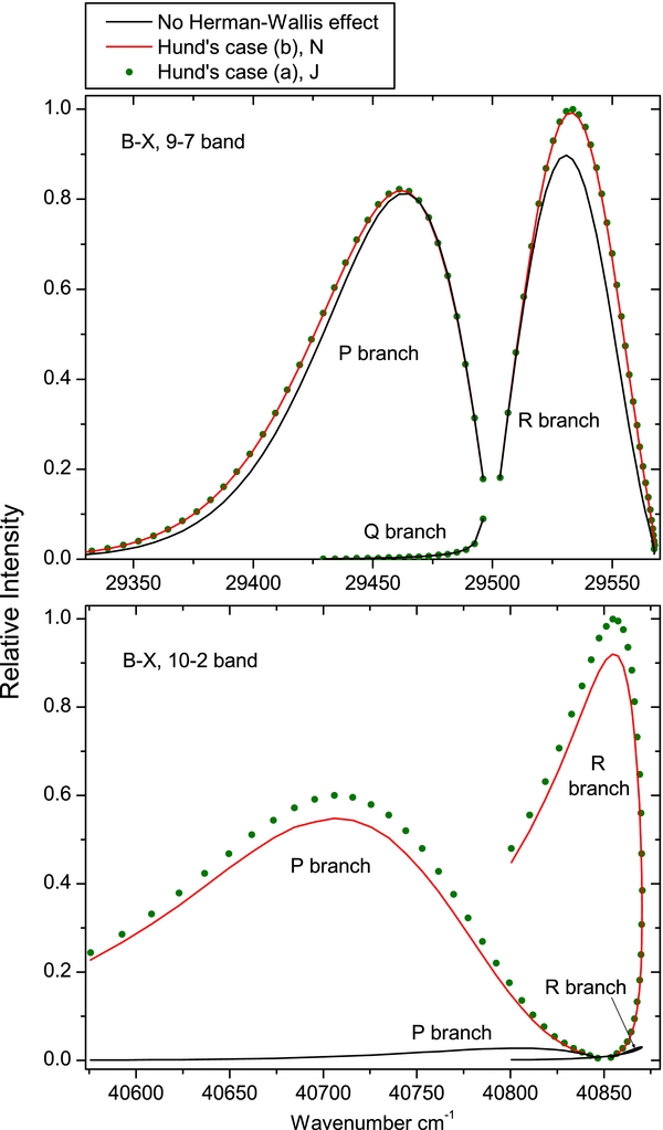
Figure 1. Relative intensities of the CN B2Σ+–X2Σ+, 9–7 and 10–2 bands. The black lines are calculated by using only one TDM matrix element for the whole band and including no Herman–Wallis effect. The green dots include the Herman–Wallis effect and the Hund's case (b) to (a) transformation of the matrix elements as described in the paper. The red lines are calculated by not performing the Hund's case transformation, and using the quantum number N instead of J to account for the Herman–Wallis effect. For both panels of the figure, the intensities have been calculated using a rotational temperature of 500 K, showing J up to 30.5. The 9–7 band was used as one example as this has the largest Herman–Wallis effect for any observed band of the B2Σ+–X2Σ+ system. The 10–2 band is a typical example of the extent of the effect for the very weak bands.
Download figure:
Standard image High-resolution image3.2.1. The A2Π–X2Σ+ System
For the calculation of line strengths of the A2Π–X2Σ+ transition of CN, the equilibrium constants in Table 2 were used as input to the  program. The potential curves (turning points) were then employed in level along with the TDM,
  , derived from high level ab initio calculations described above (Table 3).
For most vibrational bands of the CN A2Π–X2Σ+ system, the Herman–Wallis effect is calculated to be relatively small (∼5%), but for some weaker bands the effect is large. The largest difference between the matrix elements for reported rotational transitions within a vibrational band and the reference matrix element for that band (the denominator in Equation (8); the maximum Herman–Wallis effect) is 8% for the 0–0 band, 5% for the 6–8 band, and 67% for the 4–5 band (the greatest difference for an observed band). It is above 50% for several unobserved bands and one observed band. It was therefore decided that the effect should be included in our calculations.
In calculating the centrifugal part of the potential, (N(N + 1) − Λ2)ℏ/2μr2, Λ = 1 is used by level for the A2Π state. The effect of using Λ = 1 as opposed to Λ = 0 is mostly small (<0.5%), but for some bands it has a large effect. The bands in which this effect is large are mostly ones where the vibrational overlap is very small, and therefore any small alteration in the wavefunctions is more likely to cause a disproportionally large change in the overlap. The extent to which this change occurs has been investigated before (Le Roy & Vrscay 1975), where a formula for its prediction, using rotational constants and vibrational spacings, was presented. It can also be seen from the centrifugal term that Λ will have more of an effect at lower J-values.
3.2.1.1. Conversion to Hund's case (a) matrix elements
The CN A2Π state is Hund's case (a) at low J and changes toward Hund's case (b) with increasing J, so it is not possible to avoid a case (a)–case (b) transformation at some point in the calculation. For example, in the v = 0 level, B = 1.707 cm−1, A = −52.65 cm−1 and |BJ| ≈ |A| at J = 31. Given the level output, Equation (11) is used to calculate the  factors. For a particular combination of J-values, say J' = 7.5 and J'' = 8.5, the sum will require three transition moments from level with N'–N'' equal to 7–8, 8–8, and 8–9 (the sum formally includes N'–N'' = 7–9 but this violates the selection rule on N, and so its contribution calculated in Equation (11) is equal to zero).
This equation must be used for each possible combination of J', Ω', J'', and Ω'', and for a particular J', J'' there are four possible combinations of Ω that have non-zero matrix elements, corresponding to <Ω', Λ', Σ'|Ω'', Λ'',Σ''> = <+1.5, +1, +0.5|+0.5, 0,+0.5>, <−1.5, −1, −0.5|−0.5, 0, −0.5>, <+0.5, −1, −0.5|+0.5, 0, +0.5> and <−0.5, +1, +0.5|−0.5, 0, −0.5>. The first and second are in fact symmetry related as the matrix element is invariant to reversal of the signs of all the projections, as are the third and fourth. This means that the resulting matrix elements will be the same for the ones involving the Ω = ±1.5 spin component, and for the Ω = ±0.5 spin component.
The net effect of the transformation between N and J is that the dipole moment for a particular J is a (weighted) average of the dipole moment for a few values of N. As the dipole moment is only varying slowly with N, the functions of N and J are very similar, and this transformation only introduces a small correction in this case, as shown in Figure 1.
3.2.1.2. Accounting for the Herman–Wallis effect
The Herman–Wallis factors,  values (Equation (8)) are calculated using the new Hund's case (a) matrix elements. These
  values can be expressed as a polynomial according to the following equation:
There are six possible versions of this equation for the A2Π–X2Σ+ transition, two for each change in J, corresponding to the two possible spin components, Ω = ±0.5 and Ω = ±1.5, in the A2Π state. The six different polynomials for each band were fitted to Equation (12) with effective polynomial orders (which were adjusted to give a good fit), using TDM matrix elements up to the highest reported J-values, where  is J'' for ΔJ = −1, J''−Ω' for ΔJ = 0, and J''+1 for ΔJ = +1. The resulting coefficients (C, D, E, etc.; six sets for each band) were input into pgopher along with the reference TDM matrix elements (the denominator in Equation (8); these are available from the authors on request). pgopher multiplies
  by the appropriate polynomial value according to the value of
  , ΔJ and the spin component for each transition.
Please note that this differs from the standard definition of the Herman–Wallis effect (Bernath 2005), and so the coefficients calculated here are not standard. The subscripts "TDM" and "J'Ω'JΩ" are present to indicate this.
3.2.1.3. Output of the calculations
The final output of this calculation consists of line positions, Einstein A-values and f-values for 295 possible vibrational bands (63 observed), and rotational lines with J up to between 25.5 and 120.5, depending on the band (Table 4; see the online line list header for a detailed description of which lines are reported). Using the Einstein A-values obtained from this calculation, the radiative lifetimes for some lower vibrational levels (v = 1–4) of the A2Π state were calculated (as described in the following sections) and compared with the available experimental and theoretical lifetimes (see Table 5).
Table 4. List of Observed and Calculated Positions and Calculated Intensities of the CN A2Π–X2Σ+ and B2Σ+–X2Σ+ Systems, and X2Σ+ State Rovibrational Transitions
| eS' | eS'' | v' | v'' | J' | J'' | F' | F'' | p' | p'' | N' | N'' | Observed | Calculated | Residual | E'' | A | f | Description |
|---|---|---|---|---|---|---|---|---|---|---|---|---|---|---|---|---|---|---|
| A | X | 0 | 0 | 1.5 | 2.5 | 1 | 1 | e | e | NaN | 2 | 9082.98330 | 9082.9702 | 0.01313 | 11.3536 | 7.685729E+3 | 9.310961E−5 | pP1(2.5) |
| A | X | 0 | 0 | 2.5 | 3.5 | 1 | 1 | e | e | NaN | 3 | 9079.91520 | 9079.8980 | 0.01723 | 22.7030 | 1.152579E+4 | 1.571904E−4 | pP1(3.5) |
| A | X | 0 | 0 | 3.5 | 4.5 | 1 | 1 | e | e | NaN | 4 | 9076.35990 | 9076.3587 | 0.00119 | 37.8337 | 1.405716E+4 | 2.046548E−4 | pP1(4.5) |
| A | X | 0 | 0 | 4.5 | 5.5 | 1 | 1 | e | e | NaN | 5 | 9072.35580 | 9072.3561 | −0.00032 | 56.7451 | 1.596585E+4 | 2.423418E−4 | pP1(5.5) |
| A | X | 0 | 0 | 5.5 | 6.5 | 1 | 1 | e | e | NaN | 6 | 9067.89420 | 9067.8947 | −0.00046 | 79.4362 | 1.751230E+4 | 2.736789E−4 | pP1(6.5) |
Notes. eS = electronic state, p = parity. In the A state, F = 1 refers to Ω = 0.5, and F = 2 to Ω = 1.5. In the B and X states, F = 1 refers to e parity, and F = 2 to f parity. Observed = observed transition position (= "NaN" if line not observed in any study). Calculated = Position calculated by pgopher. Residual = observed - calculated position. E'' = lower state energy calculated by pgopher (relative to v'' = 0 band origin). A = Einstein A. f = f-value.
Only a portion of this table is shown here to demonstrate its form and content. A machine-readable version of the full table is available.
Download table as: DataTypeset image
Table 5. Comparison of Lifetimes (in μs) with the Selected Experimental and Theoretical Lifetimes of the v = 0–4 Vibrational Levels of the CN A2Π State
| v | This Work | Experimental | Theoretical | ||||||||
|---|---|---|---|---|---|---|---|---|---|---|---|
| A2Π1/2 | A2Π3/2 | TS | LHH | DEL | J | KWHC | BLT | LGR | CH | LSA | |
| (Ref 1) | (Ref 2) | (Ref 3) | (Ref 4) | (Ref 5) | (Ref 6) | (Ref 7) | (Ref 8) | (Ref 9) | |||
| 0 | 11.08 | 11.29 | 8.50 ± 0.5 | ... | 3.83 ± 0.5 | ... | 11.16 | 11.2 | 11.3 | 11.1 | 8.1 |
| 1 | 9.60 | 9.76 | 8.02 ± 0.6 | ... | 4.05 ± 0.4 | 7.29 ± 0.2 | 9.71 | 9.7 | 9.6 | 9.6 | 7.0 |
| 2 | 8.53 | 8.66 | 6.67 ± 0.6 | 6.96 ± 0.3 | 3.98 ± 0.4 | 7.05 ± 0.3 | 8.66 | 8.6 | 8.4 | 8.6 | 6.3 |
| 3 | 7.73 | 7.84 | 5.50 ± 0.5 | 5.09 ± 0.2 | 4.20 ± 0.4 | 6.95 ± 0.3 | 7.87 | 7.8 | 7.6 | 7.2 | 5.7 |
| 4 | 7.12 | 7.21 | 4.70 ± 0.2 | 3.83 ± 0.3 | 4.35 ± 0.4 | 6.58 ± 0.4 | 7.25 | 7.2 | 6.9 | 6.7 | 4.9 |
References. (1) Taherian & Slanger 1984; (2) Lu et al. 1992; (3) Duric et al. 1978; (4) Jeunehomme 1965; (5) Knowles et al. 1988; (6) Bauschlicher & Langhoff 1988; (7) Lavendy et al. 1984; (8) Cartwright & Hay 1982; (9) Larsson et al. 1983.
Download table as: ASCIITypeset image
3.2.2. The B2Σ+–X2Σ+ System
The calculations for the B2Σ+–X2Σ+ transition were performed in a similar manner as described for the A2Π–X2Σ+ transition. In this case a 1Σ–1Σ transition was calculated by level. The Herman–Wallis effect was again included as it is of a similar magnitude as the A2Π–X2Σ+ system. For example, the maximum Herman–Wallis effect (defined in Section 3.2.1) is 0.4% for the 0–0 band, 10% for the 6–3 band, and 42% for the 9–7 band (the greatest difference for an observed band). For several of the unobserved bands, this difference is above 1000%.
The Hund's case (b) matrix elements calculated by level were again converted to the Hund's case (a) version for input into pgopher, using Equation (11). Here, only three polynomials were required to be fitted to Equation (12) for each band, as there is only one spin component in both states.
The final line list (Table 4) consists of line positions and intensities for 253 bands of this transition with v' = 0–15, v'' = 0–15, and J up to between 25.5 and 70.5, depending on the band. The lifetimes of the B2Σ+ state levels calculated using the Einstein A-values agree well with the values obtained in previous experimental and theoretical studies.
3.2.3. The X2Σ+ Rovibrational Transitions
The main focus of this paper was to calculate intensities for the two electronic transitions mentioned. As this involved the calculation of a dipole moment function and a potential energy curve for the X2Σ+ ground state, intensities were also calculated and reported for the rovibrational and rotational transitions within the ground state. The calculations for these transitions were the same as those for the B2Σ+–X2Σ+ system, but with the upper state wavefunctions replaced by X2Σ+, and using the X2Σ+ state dipole moment function as opposed to the TDM function. Again, the Herman–Wallis effect was included, as the maximum effect (defined in Section 3.2.1) was more than 5% for most bands. For example, it is 7.0% for the purely rotational transitions, 81% for the 2–0 band (the greatest difference for an observed band) and above 100% for several of the unobserved bands. The final reported line list (Table 4) contains line positions and intensities for 253 bands of rovibrational transitions with v = 0–15, and J up to between 25.5 and 120.5, depending on the band. Einstein  values have been calculated and compared to previous values in Table 6.
Table 6. Comparison of Current and Previous Einstein  Values for Several Vibrational Bands within the X2Σ+ Ground State of CN
| Band | Einstein  (s−1) (s−1) |
|
|---|---|---|
| Langhoff & Bauschlicher (1989) | Our Value | |
| 1–0 | 13.02 | 8.85 |
| 2–1 | 24.20 | 16.5 |
| 3–2 | 33.77 | 22.9 |
| 4–3 | 41.92 | 28.2 |
| 5–4 | 48.81 | 32.3 |
| 2–0 | 1.75 | 0.661 |
| 3–1 | 4.88 | 2.33 |
| 4–2 | 9.12 | 5.02 |
| 5–3 | 14.22 | 8.43 |
| 3–0 | 0.10 | 0.00563 |
| 4–1 | 0.38 | 0.0404 |
| 5–2 | 0.95 | 0.180 |
Download table as: ASCIITypeset image
3.3. Vibrational  and Values


The  values for each vibrational band of the two transitions were calculated by adding the rotational Einstein A-values for all possible transitions within the relevant band originating from the J' = 1.5 level of the A2Π3/2 spin component in the case of the A2Π3/2–X2Σ+ sub-bands and J' = 0.5 of the A2Π1/2 component in the case of the A2Π1/2–X2Σ+ sub-bands. We have found that the
  values for the A2Π1/2–X2Σ+ and A2Π3/2–X2Σ+ sub-bands are slightly different. This difference is mainly due to the wavenumber difference of the two sub-bands. As can be noted from Equation (3), AJ'→J" ∝ ν3; therefore, the AJ'→J" values of the two spin components can be related by the equation
After conversion from one spin component to the other using the above equation, the  values of the two sub-bands become almost identical. The Einstein
  values for individual bands have been used to calculate the oscillator strength (
 ) for different bands using the equation
where δ0, Λ = 1 for a 2Σ+ state and 0 for a 2Π state. In this calculation, the wavenumber of the qQ2(0.5) line for the A2Π1/2–X2Σ+ sub-band and the rR1(0.5) line for the A2Π3/2–X2Σ+ sub-band, located close to the band origins, were used in the above equation. We have computed the Einstein coefficients  and oscillator strengths
  for 290 bands of the red system with v' = 0–22 and v'' = 0–15, 250 bands of the B2Σ+–X2Σ+ transition with v = 0–15 for both states, and 120 bands of the rovibrational transitions within the X2Σ+ state with v = 0–15. The calculated
  and
and  values are provided in Table 7. The final line list including line positions and their AJ'-J" and fJ'-J" values are provided in Table 4.
Table 7. The Vibrational  and
and  Values of the CN A2Π–X2Σ+ and B2Σ+–X2Σ+ Systems and X2Σ+ State Vibrational Transitions
| Electronic System | v' | v'' | Upper Spin Component | |||
|---|---|---|---|---|---|---|
| 2Π1/2 | 2Π3/2 | |||||
 |
 |
 |
 |
|||
| A2Π–X2Σ+ | 0 | 0 | 6.595(+4) | 2.366(−3) | 6.483(+4) | 2.350(−3) |
| A2Π–X2Σ+ | 0 | 1 | 2.193(+4) | 1.305(−3) | 2.145(+4) | 1.293(−3) |
| A2Π–X2Σ+ | 0 | 2 | 2.263(+3) | 2.626(−4) | 2.195(+3) | 2.595(−4) |
| A2Π–X2Σ+ | 0 | 3 | 7.333(+1) | 2.298(−5) | 6.969(+1) | 2.252(−5) |
| A2Π–X2Σ+ | 0 | 4 | 2.808(−1) | 6.594(−7) | 2.437(−1) | 6.236(−7) |
Note. Numbers in parentheses indicate the exponent.
Only a portion of this table is shown here to demonstrate its form and content. A machine-readable version of the full table is available.
Download table as: DataTypeset image
3.4. Radiative Lifetimes of the A2Π and B2Σ+ States
The radiative lifetime of a vibrational level of the A2Π1/2 component was calculated by taking the reciprocal of the sum of the Einstein A-values of all possible transitions originating from J' = 0.5 of that vibrational level. Similarly, the lifetime of an A2Π3/2 vibrational level was calculated by taking the reciprocal of the sum of the A-values of all the transitions from that vibrational level, the 2Π3/2 spin component and with J' = 1.5. The radiative lifetimes of both spin components of the A2Π state are provided in Table 5. The lifetimes of v = 0–5 in the B2Σ+ state are provided in Table 8. Values from some selected experimental and theoretical studies of the two transitions have also been provided in these tables for comparison.
Table 8. Comparison of Calculated Lifetimes (in ns) with the Available Experimental and Theoretical Lifetimes of the v = 0–5 Vibrational Levels of the CN B2Σ+ State
| v | This Work | Experimental | Theoretical | ||||||
|---|---|---|---|---|---|---|---|---|---|
| DEL | J | LB | NSH | BLT | KWHC | LSA | CH | ||
| (Ref 1) | (Ref 2) | (Ref 3) | (Ref 4) | (Ref 5) | (Ref 6) | (Ref 7) | (Ref 8) | ||
| 0 | 62.74 | 66.2 ± 0.8 | 65.6 ± 1.0 | 60.8 ± 2.0 | 65.0 ± 2.0 | 62.69 | 60.73 | 66.80 | 62.29 |
| 1 | 62.97 | 66.3 ± 0.8 | ... | ... | ... | 63.25 | 61.21 | 66.63 | 62.88 |
| 2 | 63.46 | 64.3 ± 2.0 | ... | ... | ... | 64.19 | 61.97 | 67.10 | 63.67 |
| 3 | 64.25 | 65.6 ± 3.0 | ... | ... | ... | 65.52 | 63.13 | 68.22 | 64.84 |
| 4 | 65.39 | 68.2 ± 4.0 | ... | ... | ... | 67.23 | 65.00 | 69.72 | 66.42 |
| 5 | 66.95 | 67.3 ± 5.0 | ... | ... | ... | 69.32 | 66.44 | 71.43 | 68.42 |
References. (1) Duric et al. 1978; (2) Jackson 1974; (3) Luk & Bersohn 1973; (4) Nishi et al. 1982; (5) Bauschlicher & Langhoff 1988; (6) Knowles et al. 1988; (7) Larsson et al. 1983; (8) Cartwright & Hay 1982.
Download table as: ASCIITypeset image
As the Herman–Wallis effect has been included, we also observed a change in the lifetimes with J. For all of the vibrational levels in the A2Π state the lifetime increases with increasing J, and the higher the vibrational level, the smaller the relative increase of the lifetime per J level. In the X2Σ+ state, the opposite is observed. In the B2Σ+ state, the lifetime decreases with J at lower vibrational levels, but increases with J at higher vibrational levels.
Since we did not observe the B2Σ+–A2Π transition in our experiment, we did not take into account the contribution of this transition to the lifetime of the B2Σ+ state. Bauschlicher & Langhoff (1988) have found that the inclusion of this transition lowers the lifetime of the B2Σ+ state by ∼1%.
4. RESULTS AND DISCUSSION
4.1. The A2Π State
There is generally good agreement between other theoretical values and our calculated A2Π1/2–X2Σ+ oscillator strengths. For example, Knowles et al. (1988) have predicted f3'0" = 3.34 × 10⁻⁴, compared to 3.35 × 10⁻⁴ predicted by Bauschlicher & Langhoff (1988). The corresponding values from our calculation agree well, as f3'0" = 3.40 × 10⁻⁴ for A2Π1/2 and f3'0" = 3.39 × 10⁻⁴ for A2Π3/2. A value of f3'0" = 4.58 × 10⁻⁴ was calculated by Larsson et al. (1983) but it was pointed out by Gredel et al. (1991) and Bakker & Lambert (1998) that the f-values of Larsson et al. (1983) were probably too large. Based on the calculations by Knowles et al. (1988) and Bauschlicher & Langhoff (1988), Bakker & Lambert (1998) have adopted the following  values with a small correction: f0'0" = 23.7 × 10⁻⁴, f1'0" = 19.1 × 10⁻⁴, f2'0" = 9.0 × 10⁻⁴, f3'0" = 3.3 × 10⁻⁴, and f4'0" = 1.1 × 10⁻⁴. These values are in very good agreement with our values of f0'0" = 23.60 × 10⁻⁴, f1'0" = 19.15 × 10⁻⁴, f2'0" = 9.15 × 10⁻⁴, f3'0" = 3.39 × 10⁻⁴, f4'0" = 1.10 × 10⁻⁴ (values shown are for the A2Π1/2 component). Adamczak & Lambert (2013) have used the red system lines in their N abundance analysis of weak G-band stars. In this study they have used a line list of the red system provided by B. Plez (2011, unpublished data), which used the
  values recommended by Bakker & Lambert (1998). The wavelengths of the useful lines were re-computed from energy levels given by Ram et al. (2010a, 2010b).
Although the calculated values agree well with the values obtained from several theoretical calculations for the A2Π state, they were significantly larger than the most recent experimental lifetimes (Taherian & Slanger 1984; Lu et al. 1992). Also, the experimental lifetimes of the A2Π state measured by different groups do not agree with each other, as can be seen in Table 5. Among the experimental values, the lifetimes reported most recently by Taherian & Slanger (1984) and Lu et al. (1992) have better agreement. Lifetimes of 8.5 ± 0.05, 8.02 ± 0.6, 6.67 ± 0.5, 5.5 ± 0.5, and 4.70 ± 0.2 μs have been reported for v = 0, 1, 2, 3, and 4, respectively, by Taherian & Slanger (1984). Unfortunately, Lu et al. (1992) did not determine the lifetimes for v = 0 and 1 for the A2Π state, but have provided the values 6.96 ± 0.3, 5.09 ± 0.2, and 3.38 ± 0.2 μs for v = 2, 3, and 4, respectively. Their values for v = 2 and 3 agree within their quoted error with the values of Taherian & Slanger (1984). Our A2Π1/2 (A2Π3/2) lifetimes are 11.08 (11.29), 9.60 (9.76), 8.53 (8.66), 7.73 (7.84), and 7.11 (7.21) μs for v = 0, 1, 2, 3, and 4, respectively. If the dipole moment function is increased by 15%, these values become 8.38 (8.54), 7.27 (7.38), 6.45 (6.55), 5.85 (5.93), and 5.38 (5.45) μs. These modified values agree better with the lifetimes reported by Taherian & Slanger (1984) and Lu et al. (1992), as well as the theoretical values of Larsson et al. (1983). However, there is no basis for such an adjustment.
The high level ab initio calculations (except Larsson et al. 1983) of lifetimes agree with each other, and given the excellent quality of the calculations we do not think that the ab initio values would change with an even higher level method. There are potentially problems with the experimental work, of which the most serious is collisional population transfer as discussed by Lu et al. (1992), which would reduce the experimental lifetimes. More experiments are needed, for example, on cold molecules in a collisionless environment with selective excitation of the upper state levels.
4.2. The B2Σ+ State
The calculated lifetimes of the B2Σ+ state agree well with the known experimental and theoretical values reported from previous studies. In particular, the present values of 62.74, 62.97, 63.46, 64.25, 65.39, 66.95 ns agree within ∼5% with the experimental values of Duric et al. (1978), obtained with the high frequency deflection technique. The theoretical calculations of the oscillator strength of the B2Σ+–X2Σ+ bands by Knowles et al. (1988) and Bauschlicher & Langhoff (1988) predict f0'0" = 0.0345 and 0.0335, respectively, compared to f0'0" = 0.0337 in the present study. An earlier calculation by Larsson et al. (1983) has provided a value of f0'0" = 0.0324. Since the experimental lifetimes of the B2Σ+ state (Nishi et al. 1982; Duric et al. 1978; Jackson 1974; Luk & Bersohn 1973) agree well with theoretical results (Cartwright & Hay 1982; Larsson et al. 1983; Lavendy et al. 1984; Knowles et al. 1988; Bauschlicher & Langhoff 1988), an average value of f0'0" = 0.033 was adopted by Bakker & Lambert (1998) in their study of the 12CN and 13CN lines of the red and violet systems in the spectrum of the post-asymptotic giant branch star HD 56126. Our value of f0'0" = 0.0337 also supports the value adopted by Bakker & Lambert (1998). The much shorter lifetime of the B2Σ+ state means that the experimental measurements will be much less sensitive to neglected loss mechanisms in the excited state, so the existence of discrepancies in only the A2Π state lifetimes is not surprising.
4.3. The X2Σ+ State
The calculated Einstein  values have been compared to those of Langhoff & Bauschlicher (1989) in Table 6. Our values are noticeably smaller; they are around 2/3 of the 1989 values for the Δv = 1 sequence, and as low as about 1/10 in one case (the 4–1 band). The reason for this can be seen in Figure 2, which shows the difference between the 1989 dipole moment function and ours. The differences here cause the discrepancies in the final Einstein
  values. To confirm this, the full calculations described in this paper were performed using the 1989 dipole moment function, and the Einstein
  values were calculated to be almost identical to those reported by Langhoff and Bauschlicher.
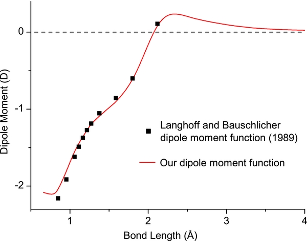
Figure 2. Theoretical dipole moment functions for the CN X2Σ+ ground state.
Download figure:
Standard image High-resolution image4.4. Validation of Computed Results
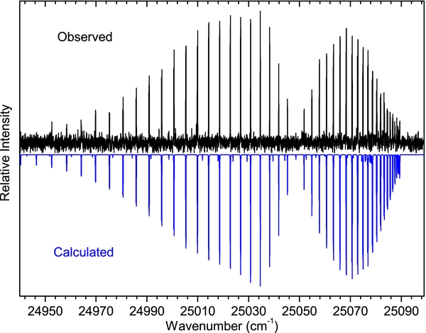
The spectrum of the A2Π–X2Σ+ transition is spread over a wide wavenumber range (from 4000–21,500 cm−1), so it was recorded in two parts with different experimental conditions. As mentioned earlier, spectra were observed in emission from an active nitrogen afterglow source in which energy transfer takes place from the metastable triplet A3Σu+ and vibrationally excited ground state of N2 to higher vibrational levels of the excited and ground states of CN. In such a case, the vibrational and rotational temperatures are very different, and because of incomplete relaxation the concept of a vibrational temperature has little meaning. In this case, we started by adjusting the Lorentzian and Gaussian contributions to linewidths in pgopher to find the best match between the observed and calculated line shapes. Next, the rotational temperature was estimated by monitoring the intensity distribution of a large number of rotational lines in a branch while varying the rotational temperature in small steps. A value of 500 K was estimated for the A2Π–X2Σ+ bands in the 4000–12,000 cm−1 region. In order to simulate the spectrum of sequence bands, the rotational temperature was held fixed but the vibrational temperature was adjusted in steps. It was found that a vibrational temperature of 15,000 K produced a reasonable correspondence between the observed and simulated spectra. A part of the spectrum of the Δv = −1 sequence of the A2Π–X2Σ+ transition is presented in Figure 3, over a range of about 2000 cm−1. As can be seen, the intensity of the 0–1, 1–2, 2–3, 3–4, 4–5, and 5–6 bands decrease rapidly and the 5–6 band is almost absent in the observed and simulated spectra. The higher vibrational bands again appear gradually in both the observed and simulated spectra. An expanded portion of the spectrum of the 0–1 band near the R2 head is presented in Figure 4, and the sR21 branch of the 1–0 band is provided in Figure 5, showing good agreement between the observed and simulated spectra.
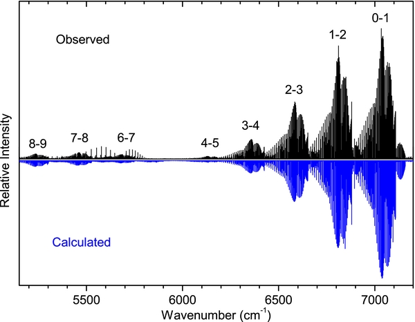
Figure 3. Comparison of the observed (upper) and simulated (lower) spectra of the Δv = −1 sequence of the A2Π–X2Σ+ transition of CN. The unmarked emission lines near the 6–7 and 7–8 bands are vibration–rotation lines of the 2–0 overtone of HCl, present as an impurity. The absence of 5–6 band in both spectra is consistent with the very small Franck–Condon factor calculated by level.
Download figure:
Standard image High-resolution image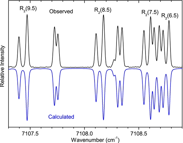
Figure 4. Comparison of a part of the observed (upper) and simulated (lower) spectra of the A2Π–X2Σ+, 0–1 band near the R2 head showing a very good correspondence between the two spectra.
Download figure:
Standard image High-resolution image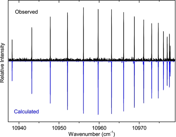
Figure 5. Comparison of the observed (upper) and simulated (lower) spectra of the A2Π–X2Σ+, 1–0, sR21 branch.
Download figure:
Standard image High-resolution imageFor the B2Σ+–X2Σ+ transition, a similar comparison is more difficult because of the formation of a head of band heads in the different sequences. Also, interactions between the excited state and nearby perturbing levels cause abnormal intensities in some of the vibrational bands so the relative intensity of the simulated bands differs somewhat from the observations. For this transition, rotational and vibrational temperatures of 300 K and 3400 K result in a reasonable match between the observed and simulated spectra. A section of the 13–13 band showing very good agreement between observed and simulated spectra is provided in Figure 6.
Figure 6. A section of the observed (upper) and simulated (lower) spectra of the B2Σ+–X 2Σ+, 13–13 band comparing the intensity distribution of the R and P branches.
Download figure:
Standard image High-resolution image
5. SUMMARY
TDM functions for the A2Π–X2Σ+ and B2Σ+–X2Σ+ systems and a dipole moment function for the X2Σ+ state of CN were calculated, and employed in the program level to calculate TDM matrix elements. An equation was derived to convert matrix elements from Hund's case (b) to (a), their J dependence was quantified and the effect of rotation on the matrix elements was included before their input into pgopher. This program was used to calculate Hönl–London factors and Einstein A coefficients. A line list consisting of line positions, Einstein A coefficients and f-values for 290 bands of the A2Π–X2Σ+ transition with vibrational levels v' = 0–22, v'' = 0–15, 250 bands of the B2Σ+–X2Σ+ transition with v' = 0–15, v'' = 0–15 and 120 bands of the rovibrational transitions within the X2Σ+ state with v = 0–15 has been generated. The Einstein A-values have been used to compute radiative lifetimes in the A2Π and B2Σ+ states. The calculated f-values of the two transitions agree with the theoretical values of Knowles et al. (1988), Bauschlicher & Langhoff (1988), and Cartwright & Hay (1982), and the values adopted by Bakker & Lambert (1998). The A2Π state lifetimes have also been calculated with the modified TDMs (increased by 15%) which compare well with the recent experimental values for the lower vibrational levels of the A2Π state, but we recommend the use of the unmodified ab initio values. Our B2Σ+ state lifetimes and f-values have good agreement with the previously reported experimental and theoretical values as well as the values adopted values by Bakker & Lambert (1998) in their chemical abundance analyses. The Einstein  values for the X2Σ+ state rovibrational transitions are significantly smaller than previous values from Langhoff & Bauschlicher (1989), but we believe the new dipole moment function to be more accurate. To validate the calculated relative line intensities, laboratory spectra were simulated and good agreement has been found between observed and calculated spectra.
The research described here was supported by funding from the Leverhulme Trust of UK and the NASA laboratory astrophysics program. The spectra used in this work were recorded at the National Solar Observatory at Kitt Peak, USA.
APPENDIX: DERIVATION OF THE EQUATION (EQUATION (11)) FOR CONVERTING HUND'S CASE (B) MATRIX ELEMENTS TO HUND'S CASE (A) MATRIX ELEMENTS
A.1. Relationship between Hund's Case (a) and Case (b) Wavefunctions
Starting from the general relationship given by Brown & Howard (1976),

and applying the constraint K = Λ appropriate for linear molecules we have

The transformation between Hund's case (a) and (b) should be orthogonal, so we can essentially invert the transformation by inspection. Both sides are multiplied by a trial function to verify this:
Summing both sides over N gives
The last step follows from the orthogonality relationship:

given that the additional sum over γ collapses to the term with α + β + γ = 0 = α' + β' + γ. Overall

A.2. Relationship between Hund's Case (a) and Case (b) Electronic Transition Moments
For transition strengths, we require the matrix elements of the space fixed electric dipole operator:

The matrix elements of this are well known; in a Hund's case (a) basis they are
This is essentially Equation (6.320) of Brown & Carrington (2003) generalized to any value of p and q. In addition, to a first approximation the electronic matrix element  should not depend on J or Ω, but these have been added as parameters here to allow for centrifugal distortion.
A similar equation can be derived for Hund's case (b) wavefunctions:
This is a generalization of Equation (6.321) of Brown & Carrington (2003). Again the purely electronic matrix element  should not depend on N, but we allow it to do so to allow for centrifugal distortion.
We now need to relate these two using the transformation between bases derived above:

Substituting on both sides
The terms in M cancel out:
and with a little more simplification:
Λ and Λ' are the same on both sides, so the equation can be used for a single value of q:
Finally,
(Equation (11) in main text)