Introduction

It is commonly assumed that, in the steady state, the rate of melting on the wall of an englacial or subglacial conduit due to viscous dissipation balances closure of the conduit by flow of the ice (Röthlisberger, 1972; Reference ShreveShreve, 1972). Using this assumption, Röthlisberger (1972, equation (20)) derived an expression relating the pressure gradient in subglacial conduits to conduit characteristics and the steady water discharge. By integrating this equation up-glacier from the terminus, using the water pressure at the terminus as a boundary condition, he calculated water pressures as a function of distance from the terminus. His calculations of the water pressure beneath Gornergletscher, however, did not agree well with a water pressure that was measured about 1.2 km up-glacier from the terminus. To achieve agreement, Röthlisberger had to assume not only that the conduit was unusually rough, but also that the ice-viscosity parameter, B, was only 1.0 bar a^1/3, which is significantly less than the value of ~1.6bar a^1/3 that is widely accepted for temperate ice (e.g. Reference HookeHooke, 1981; Reference PatersonPaterson, 1981, p. 39; Reference Lliboutry and DuvalLliboutry and Duval, 1985, p. 215). As strain-rates are inversely proportional to the cube of the viscosity, Röthlisberger was, in effect, assuming that the basal ice was a factor of 4 softer than normal.

Reference LliboutryLliboutry (1983, p. 222) suggested that conduits close faster in zones of high pressure on the stoss sides of irregularities in the bed, and that failure to take this into account might explain the low value of B that Röthlisberger needed. Reference HookeHooke (1984, p. 185) suggested, alternatively, that Röthlisberger might have misinterpreted the water-pressure data, which, in fact, showed quite low pressures in late summer. Hooke’s calculations suggested that conduits on the down-glacier sloping bed beneath the outermost 2.2 km of Gornergletscher should be at atmospheric pressure.

Reference Iken and BindschadlerIken and Bindschadler (1986) also compared water-pressure data that they obtained from bore holes on Findelengletscher with pressures calculated using Röthlisberger’s model. They, too, found that agreement was best when they used a value of B that was substantially lower than accepted values, and suggested a number of possible causes of such enhanced plasticity. Among these were the presence of impurities or unfrozen water, the non-isotropic stress state, and the possibility of transient creep. In addition, they suggested that the flow path was probably quite sinuous, a characteristic not taken into consideration in Röthlisberger’s model.

While many of these suggestions have merit and may contribute to the high water pressures observed, we pursue here an alternative mentioned briefly by Reference LliboutryLliboutry (1983, p. 222) and by Reference Iken and BindschadlerIken and Bindschadler (1986, p. 114) but not developed by them: namely, that the channel shape assumed in the Röthlisberger model is incorrect. Specifically, we investigate the possibility that the channels are broad and low, a shape often observed at the termini of valley glaciers. Such a shape might well develop through melting low on the conduit walls during periods of low flow, and through drag on the bed which inhibits closure of the conduit near the bed. Walder (personal communication, May 1989) has also found that broad low conduits are likely to form when the bed over which the water is flowing consists of non-cohesive material that can be transported by the water. First, however, we present water-pressure data for two additional glaciers. Later we show that these data, too, cannot be explained by the Röthlisberger model as it stands.

Water-Pressure Measurements On Austdals-Breen And Storglaciären

In connection with hydro-electric development, water-pressure measurements have been made on Austdalsbreen, an outlet glacier from Jostedalsbreen, Norway. Eight holes were drilled to the base of the glacier, two a few meters apart in each of four locations (Fig. 1). Water pressures in the holes tended to increase gradually during the winter, and in some cases more rapidly in the early spring (Fig. 2). In late May or early June, pressures dropped abruptly and began to oscillate diurnally. In order to compare the measurements with calculated pressures, we have estimated the mean late-winter/early-spring water levels at each of the four locations in Figure 2 (see starred lines), and plotted these at the appropriate locations on Figure 1. Where pressures in Figure 2 exceeded the water-equivalent line, it was assumed that a local pressure, not representative of average conditions at the base of the glacier, was being measured. These parts of the record were ignored in selecting the water levels to plot in Figure 1.

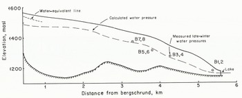
Fig. 1. Longitudinal section of Ausldalsbreen showing locations of bore holes, mean late-winter water levels in the holes, and an hydraulic grade line calculated with к = 10m¹/³ s⁻¹. В = 1.6 bar a ¹/³, and Ω = 13.

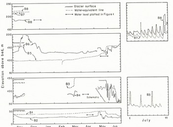
Fig. 2. Water-pressure measurements on Austdalsbreen. Locations of holes are shown in Figure 1. Gaps in record are due to periodic failure of recording system.

On Storglaciären, a valley glacier in northern Sweden, water-pressure measurements have been made in many bore holes for varying lengths of time over the past 7 years (Reference Hooke, Calla, Holmlund, Nilsson and StroevenHooke and others, 1989). A general characteristic of these measurements is that, above the riegel that lies near the middle of the ablation area (Fig. 3), water levels are almost invariably high and remarkably constant. In contrast, below the riegel, diurnal oscillations are common during the summer. However, some winter data suggest that pressures here begin to rise in the late autumn and early winter, and are relatively constant in late spring (Reference Hooke, Calla, Holmlund, Nilsson and StroevenHooke and others, 1989, fig. 3a).

Modification Of RÖthisberger’s Model

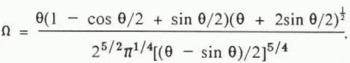
Calculations of subglacial water pressure as a function of distance from the termini of Austdalsbreen and Storglaciären were made with the use of the equation:

(1)

where dP/dx is the pressure gradient along the course of the conduit; G = (P/dx+ ρ_w gtan β), where ρ _w is the density of water, and g is the acceleration due to gravity; D is a constant involving, among other quantities, the densities of ice and water, the latent heat of fusion, and g; к is the reciprocal of the Manning roughness of the conduit; n, taken to be 3 here (Reference HookeHooke, 1981), and B are the constants in Glen’s flow law for ice, έ = (τ/B)ⁿ; Q is the water discharge; ß is the slope of the bed, taken as positive when the bed slopes downward in the direction of flow; ΔP is the difference between the pressure in the ice adjacent to the conduit and that in the water in the conduit; and Ω is a conduit-shape factor which is explained below. This equation is identical to Röthlisberger’s (1972) equation (20) except for the term Ω.

If we approximate the shapes of conduits by the space between the chord of a circle and the arc subtended by that chord (Fig. 4), the cross-sectional area of the conduit, A, is r ²(θ - sin θ)/2, and the wetted perimeter, p, is r(θ + 2sin θ /2). Röthlisberger’s development can be modified to reflect this conduit shape if an expression can be obtained for the closure of such conduits.

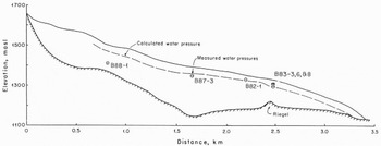
Fig. 3. Longitudinal section of Slorglaciären showing locations of bore holes, mean water levels in the holes, and an hydraulic grade line calculated with к = 10m¹/³s⁻¹. B = 1.6 bar a¹/³, and Ω = 150. Hole B88–1 was ≈200 m from the line of the profile, at a point where the glacier was ≈30 m thicker than shown. Furthermore, the water-level measurement was made on 30 June 1988. 10–15 d after the lower part of the glacier had accelerated into its summer regime. For all these reasons, the measurement may not be representative of winter conditions.

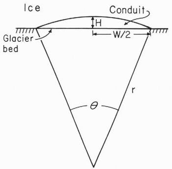
Fig. 4. Sketch showing conduit geometry assumed.

We suspected that the closure rate might lie between limiting values obtained by replacing the conduit radius inNReference Nye ye’s (1953) theory first with the conduit height, H (Fig. 4), and then by its half-width, W/2. We thus used the mean of these two lengths in place of the radius in the relation for conduit closure in Röthlisberger’s (1972, equation (6)) theory. This leads to Equation (1) with

(2)

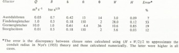
To test our approximation for the closure rate, we modelled numerically the closure of conduits such as that in Figure 4, using a finite-element program (Reference HansonHanson, 1990). As will be discussed further below, the discrepancy between the closure rate obtained by using (H + W/2)/2 to approximate the conduit radius in Nye’s theory and the rate obtained from the numerical calculation averaged 22%, and was 53% in the worst of the four cases studied. Thus, for the purposes at hand, this approximation seems adequate.

It is convenient to express Ω in terms of the fraction, δ, by which the accepted value of B must be multiplied to obtain agreement between calculated and observed water pressures, thus:

δ is plotted as a function of θ in Figure 5.

By choosing θ < η, an observed pressure gradient or hydraulic grade line can be modelled without reducing B below the accepted value of 1.6 bar a¹/³. For example, Röthlisberger used a value of B of 1.0 bar a¹/³ (δ = 0.61). This would be equivalent to a value of θ of about 36° (Fig. 5; Table I). Similarly, the value of B that gives the best fit between Reference Iken and BindschadlerIken and Bindschadler’s (1986) observed (figs 4 and 5) and calculated (Fig. 4) water pressures was about 0.3bara¹/³ (δ = 0.18), which would correspond to θ ≈ 2°.

Fig. 5. Relationship between θ and the factor, δ. by which B must be reduced ία obtain the same hydraulic grade line.

It should be noted that, contrary to the above hypothesis, a semi-circular or parabolic subglacial conduit has been observed beneath Gornergletscher a short distance down-stream from the Gornersee (Röthlisberger, 1972, fig. 11). Lliboutry (personal communication, December 1989) suggests that this may be because this particular conduit carries much larger discharges than those considered elsewhere in this paper. Alternatively, this conduit may have developed under non-steady-state flow conditions associated with the draining of the Gornersee. When melting greatly exceeds closure, conduits will be full and the effects of drag on the bed during closure of the conduit will be negligible. As noted, both of these effects will favor semi-circular rather than broad, low conduit cross-sections.

Table I. Channel characteristics

Comparison With Measurements On Austdalsbreen And Storglaciaren

Hydraulic grade lines were calculated for Austdalsbreen and Storglaciären using Equation (1). Following Röthlisberger, the conduit roughness was taken to be 10m¹/³s⁻¹ in both cases. The calculation for Austdalsbreen assumed a late-winter discharge of 0.05 m³ s⁻¹, while that for Storglaciären used 0.01m³s⁻¹. Both figures are estimates. Austdalsbreen terminates in a lake, so it has not been feasible to measure the winter discharge. In the case of Storglaciären, late-winter discharges have been observed, but not measured. The values of θ required to obtain the agreement shown in Figures 1 and 3 were about 14 and 2°, respectively (Ω ≈ 13 and 140).

Channel Geometries

The actual geometries of the channels corresponding to the values of θ thus obtained can be calculated by first determining r (Fig. 4) from:

(3)

The resulting values of H and W are shown in Table I. The calculations suggest channels, particularly for Findelengletscher and Storglaciären, that are wider and shallower than may be reasonable. However, two ~0.5 m wide, 10 to 0>30 mm deep channels (in addition to a 0.3 m diameter semi-circular conduit) were observed at the bed of the Norwegian glacier, Bondhusbreen, beneath ~160 m of ice (Reference Hooke, Wold and HagenHooke and others, 1985, p. 392). Furthermore, the numerical modelling suggests that using (H + W/2)/2 to approximate the conduit radius in the closure-rate calculations underestimates the actual rate. Correcting for this error would increase the values of H and decrease those of W shown in Table I. Finally, we stress that neither the calculations nor the field data are sufficiently accurate to justify conclusions other than that the channels may well be several times wider than they are high.

Discussion

The mean value of θ from these four examples is ~14° ° (Ω ~13), so we will use this as a typical value for purposes of further discussion. Such a value would correspond to a reduction in B to ~0.7 bar a¹/³, or to ~40% of its normal value. This would result in a ~16x enhancement of the strain-rate.

Such enhancement could occur if the water content of the ice were in excess of 7% (Reference DuvalDuval, 1977), but this is unreasonably high. It is, for example, almost triple the highest measured by Reference Vallon, Petit and FabreVallon and others (1976, p. 24) in a 187 m core from Vallée Blanche on Mont Blanc. Softening of the ice could also be due to the presence of other impurities, but available data on the effects of different species of impurity do not appear to be extensive; a suggestion of the impurity content required to produce such a softening can be obtained from Reference Jones and GlenJones and Glen’s (1969, p. 17) experiments at –20 K on ice doped with HF, a particularly potent impurity, though not common in glacier ice. An HF concentration of 67 ppm resulted in only a five-fold increase in strain-rate, and indications were that the effect would probably decrease as the temperature rose towards the melting point. Concentrations of more common impurities are probably typically >~10ppm in temperate glaciers (Reference HarrisonHarrison, 1972, p. 26). Thus, it is unlikely that impurities alone could account for the softness of the ice.

Reference Iken and BindschadlerIken and Bindschadler (1986, p. 114) suggested that the softness of the ice might be attributed, in part, to transient creep in the changing stress field present in ice flowing over an irregular bed. This is open to question. The ice near the bed of a glacier will have recrystallized and developed a c-axis fabric with a preferred orientation. It will thus be deforming in tertiary creep. When such ice moves into a location with a different stress field, it will already have a high dislocation density and the resulting transient-creep phase lasts only about a half hour (personal communication from L. Reference NyeLliboutry, December 1989). Further-more, owing to the fabric, it is equally or perhaps more likely that the ice will be stiffer rather than softer in the new stress field. Thus, it seems unlikely that we can appeal to transient creep to explain the apparent softness of the ice around tunnels.

Reference Lliboutry and DuvalLliboutry (1983, p. 222) suggested that the apparent softness of ice around subglacial conduits might be due to enhanced closure rates on the stoss sides of irregularities on the bed. If ∆P were doubled on the stoss sides of bumps and vanished on the lee sides where ice could become separated from the bed, the enhancement could be as much as a factor of 4. This is sufficient to account for the observed water pressures beneath Gornergletscher (Reference Lliboutry and DuvalLliboutry, 1983, p. 222), but substantially more separation would be required to account for the observed water pressures on the other three glaciers. Such extensive separation is unrealistic.

Reference Iken and BindschadlerIken and Bindschadler (1986, p. 114–15) suggested that part of the discrepancy between observed and calculated subglacial water pressures can be attributed to the sinuosity of the subglacial flow paths. As dP/dx is calculated along the flow path, the more sinuous the flow path, the higher the pressure at a point a given straight line distance from the margin. To test this possibility, the computer program used to calculate the energy grade lines in Figures 1 and 3 was modified to allow the user to specify the sinuosity. With B = 1.6bar a¹/³, sinuosities of 6 and 30 were required to obtain reasonable agreement with measurements on Austdalsbreen and Storglaciären, respectively. These seem quite improbable.

Concluding Statement

Clearly, all of the above processes could be working in concert to produce the high conduit-closure rates suggested by the measured water pressures. However, rather than the ice being unusually soft, our suggestion that the conduits are broad and low, is at least as reasonable as any others that have been suggested. Furthermore, it appears that in most instances it is the only one that could, alone, account for the observed pressures. The major weakness in the development is one that pervades the theoretical literature on water pressures in subglacial channels: the need to rely on Reference NyeNye’s (1953) theory, in some form, to calculate the closure rates of the channels despite the fact that virtually all of the important assumptions that Nye made in his theoretical development are violated in the natural situation.

Acknowledgements

Many of the ideas in this paper were developed while the senior author was enjoying the hospitality of the Norwegian Water Resources and Energy Administration. The authors would like to acknowledge the role that stimulating conversations with B. Wold and other members of the Glaciology Office played in the paper. Financial support for the field work on Storglaciären was provided by the Swedish Natural Science Research Council and the U.S. National Science Foundation (DPP-8414190, DPP-8619086, and INT-8712749). Important items of permanent equipment were purchased with funds generously provided by the Wallenberg Foundation of Sweden. The critical comments of L. Lliboutry and J. Walder resulted in significant improvements in the paper.