Interannual Variability and Trends of Sea Surface Temperature Around Southern South America
 Daniela B. Risaro
 María Paz Chidichimo
 Alberto R. Piola
- 1Departamento de Oceanografía, Servicio de Hidrografía Naval, Buenos Aires, Argentina
- 2Consejo Nacional de Investigaciones Científicas y Técnicas, Buenos Aires, Argentina
- 3Departamento de Ciencias de la Atmósfera y los Océanos, Facultad de Ciencias Exactas y Naturales, Universidad de Buenos Aires, Buenos Aires, Argentina
- 4CNRS-IRD-CONICET, UBA Instituto Franco-Argentino para el Estudio del Clima y sus Impactos (UMI 3351 IFAECI), Buenos Aires, Argentina
The interannual variability and trends of sea surface temperature (SST) around southern South America are studied from 1982 to 2017 using monthly values of the Optimally Interpolation SST version 2 gridded database. Mid-latitude (30°–50°S) regions in the eastern South Pacific and western South Atlantic present moderate to intense warming (~0.4°C decade−1), while south of 50°S the region around southern South America presents moderate cooling (~ −0.3°C decade−1). Two areas of statistically significant trends of SST anomalies (SSTa) with opposite sign are found on the Patagonian Shelf over the southwest South Atlantic: a warming area delimited between 42 and 45°S (Northern Patagonian Shelf; NPS), and a cooling area between 49 and 52°S (Southern Patagonian Shelf; SPS). Between 1982 and 2017 the warming rate has been 0.15 ± 0.01°C decade−1 representing an increase of 0.52°C at NPS, and the cooling rate has been –0.12 ± 0.01°C decade−1 representing a decrease of 0.42°C at SPS. On both regions, the largest trends are observed during 2008–2017 (0.35 ± 0.02°C decade−1 at NPS and –0.27 ± 0.03°C decade−1 at SPS), while the trends in 1982–2007 are non-significant, indicating the record-length SSTa trends are mostly associated with the variability observed during the past 10 years of the record. The spectra of the records present significant variance at interannual time scales, centered at about 80 months (~6 years). The observed variability of SSTa is studied in connection with atmospheric forcing (zonal and meridional wind components, wind speed, wind stress curl and surface heat fluxes). During 1982–2007, the local meridional wind explains 25–30% of the total variance at NPS and SPS on interannual time scales. During 2008–2017, the SSTa at NPS is significantly anticorrelated with the local zonal wind (r = –0.85), while at SPS it is significantly anticorrelated with the meridional wind (r = –0.61). Our results show that a substantial fraction of the interannual variability of SSTa around southern South America can be described by the first three empirical orthogonal function (EOF) modes which explain 28, 16, and 12% of the variance, respectively. The variability of the three EOF principal components time series is associated with the combined variability of El Niño–Southern Oscillation, the Interdecadal Pacific Oscillation and the Southern Annular Mode.
1. Introduction
The variability of Sea Surface Temperature (SST), which is highly influenced by feedbacks with the atmosphere, is a sensitive indicator of climate change. Recent observation-based estimates indicate a fast increase of global SST in the past decades as part of a long-term warming of the ocean surface since the mid-nineteenth century (Rhein et al., 2013; Abram et al., 2019). Between 1993 and 2015 global mean SST has increased at a rate of 0.016 ± 0.002°C year −1 (Von Schuckmann et al., 2016), and this increasing rate persisted during 2016 (Von Schuckmann et al., 2018). Atmospheric CO2 has increased substantially since the start of the Industrial Revolution generating an imbalance of energy in the Earth and therefore warming and increased absorption of CO2 by the oceans (Ciais et al., 2014; Le Quéré et al., 2018). The majority (~93%) of the extra thermal energy in the climate system accumulates in the ocean (Rhein et al., 2013). Consequently, the ocean heat content (OHC) has increased by 370 ± 81 ZJ since the 1960s, with contributions of 62.5% in the upper ocean (0–700 m) and 28.6% in the intermediate ocean (700–2,000 m) (Ishii et al., 2017; Cheng et al., 2020; Johnson and Lyman, 2020). Ocean warming in the past decades has led to global mean sea level rise in response to the input of freshwater by melting of glaciers and ice sheets, and to a lesser extent due to ocean thermal expansion (Church et al., 2013; Nerem et al., 2018; Oppenheimer et al., 2019). Ocean warming is considered a major driver of variability, inducing changes in circulation, mixing, oxygen content and bioavailability (Oschlies et al., 2018) which may promote the expansion of oxygen minimum zones (OMZ) and a reduction of available habitat for some species, particularly temperature and chemistry-sensitive organisms (Stramma et al., 2012; Abram et al., 2019; Bindoff et al., 2019).
Documenting fine-scale variability in temperature trends is an important step in developing and understanding the impact of climate change on marine ecosystems (Doney et al., 2012; Ramírez et al., 2017). Variations in SST can affect marine species altering their physiological functions and behavior. Shifts in the spatial ranges of their distribution are expected, such as their poleward migration (Walther et al., 2002; Parmesan and Yohe, 2003; Ling et al., 2009). Changes in species abundance and composition have also been observed, particularly in phytoplankton communities (Hays et al., 2005), which may, in turn, affect oceanic primary production and thus CO2 sequestration (Beaugrand and Reid, 2003; Rivadeneira and Fernández, 2005). Improved knowledge on the space and time variability of SST and of its main drivers is of great climatic relevance in the current global climate change scenario.
The upper ocean temperature has been rising at global scale (Hartmann et al., 2013). However, there are significant regional variations in its pattern, characterized by warming hot spots (Hobday and Pecl, 2014) and also by regions where the ocean has been cooling (e.g., Muller-Karger et al., 2014). For example, one of the detected regional hotspots that is warming faster than the global average is the southwestern South Atlantic Ocean (SWA) (e.g., Hobday and Pecl, 2014). In contrast, since 1979 cooling trends occur in areas of the Southern Ocean associated with sea ice expansion Fan et al., 2014) that could respond to greenhouse forcing and a positive Southern Annular Mode trend (Kostov et al., 2018). Despite the significant impacts of SST variations on the marine environment, the nature of its long-term variability and trends, and the physical mechanisms that modulate those changes are still poorly understood. Though several studies addressed the impact of climate oscillations by teleconnection patterns in SST in mid and high latitudes in the North Atlantic Ocean (Lee et al., 2008; García-Serrano et al., 2017; Yang et al., 2018; Hardiman et al., 2019; Mezzina et al., 2020) very few have been carried out in the southern hemisphere (Meredith et al., 2008; Rodrigues et al., 2015; Garreaud et al., 2021). Observed changes in mid-latitude SST on timescales from months to years in the South Atlantic have been associated with remote atmospheric fluctuations in the tropical Pacific Ocean, particularly during El Niño events when the response in the extratropics may be due to the atmospheric bridge mechanism (Dong et al., 2006; Kayano and Capistrano, 2014; Rodrigues et al., 2015).
Here we focus our analyses on the productive Atlantic continental shelf off southern South America (70°–60°W, 40°–60°S), hereafter Patagonian Shelf (PS, after Piola et al., 2018). South of 40°S the climatological wind stress is relatively high, around 0.15 Pa (Palma et al., 2004), due to the strong westerly winds (Glorioso and Flather, 1995). Annual-mean climatological SST on the PS varies between 7°C south of ~52°S and 14°C at ~42°S with a strong seasonal cycle with ~7°C annual amplitude (Rivas, 2010). High tidal amplitude, the inflow of low-salinity water from the Magellan Strait, and persistent westerly winds force a long-term mean northeastward circulation (Palma et al., 2004, 2008; Matano et al., 2010). Offshore from the continental shelf, the mean circulation in the SWA is characterized by the northward flowing Malvinas Current (MC) which advects nutrient-rich subantarctic waters along the upper continental slope. Near 38°S, the MC encounters the southward flowing Brazil Current (BC) characterized by warm and salty subtropical waters (e.g., Gordon and Greengrove, 1986). The region where the MC and BC encounter is referred to as Brazil-Malvinas Confluence (BMC) (see mean dynamic topography (MDT) field in Figure 1A).
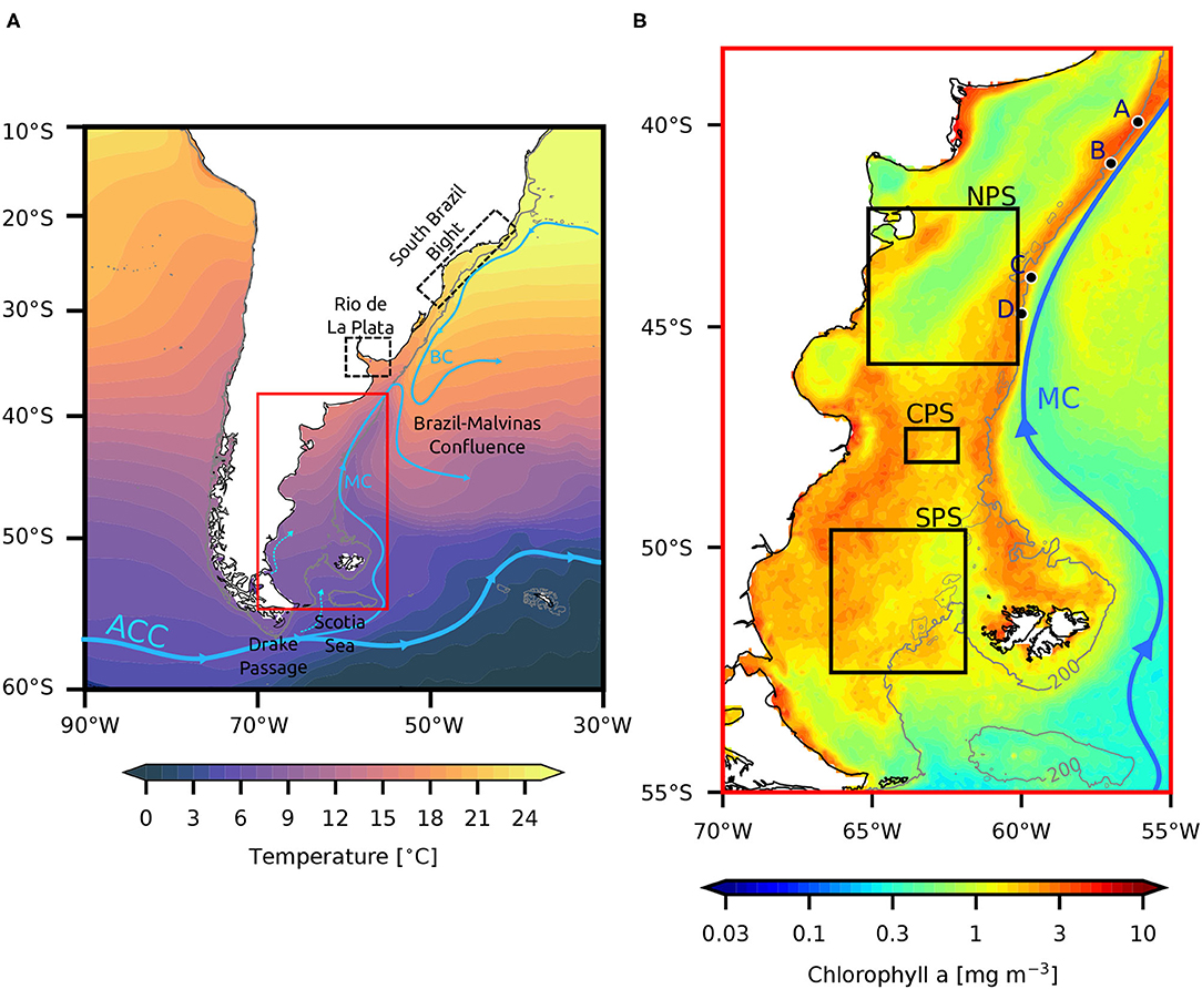
Figure 1. (A) Distribution of climatological SST between 1982 and 2017 (see Section 2.1). Overlaid light blue arrows represent the schematic circulation of the Antarctic Circumpolar Current (ACC), Malvinas Current (MC) and Brazil Current (BC), based on the climatological MDT (1993–2012) from AVISO. (B) Climatological austral summer chlorophyll-a surface distribution (2002–2017) derived from MODIS aqua with 9 km spatial resolution. Also shown is the 200 m isobath (solid gray line, data from ETOPO1). Black dots (Sites A to D) are buoy locations of in-situ wind measurements (see also Table 2). Black rectangles indicate from North to South the main regions analyzed in this study: Northern Patagonian Shelf (NPS), Central Patagonian Shelf (CPS), and Southern Patagonian Shelf (SPS) (see Section 3.2, Table 3).
The above-mentioned processes lead to stratification-destratification cycles, nutrients redistribution and retention zones that mediate one of the most productive marine ecosystems in the southern hemisphere (Bisbal, 1995; Falabella et al., 2009). Phytoplankton blooms occur during the spring over most of the shelf region and persist through the summer when the vertical stratification is intense, particularly near frontal regions (Acha et al., 2004; Romero et al., 2006) (Figure 1B). The phytoplankton productivity sustains a diverse community of species including significant fisheries and top predators that feed on and breed in its seas (e.g., Acha et al., 2004). SST variability in this region could lead to changes in the vertical stratification and therefore affect the timing and persistence of these blooms (Pecl et al., 2014; Gianelli et al., 2019).
In this study, we describe the linear trends and interannual variability of SST on the PS between 1982 and 2017, and explore the possible links with local and remote atmospheric forcing processes. We describe the observed spatial distribution of long-term trends and interannual SST fluctuations focused on areas of significant warming and cooling. To understand the forcing mechanisms of the observed SST fluctuations, we analyzed the relationships between SST anomalies and local winds, air-sea heat fluxes and sea level pressure, and with teleconnection patterns associated with global ocean-atmospheric oscillations, i.e., Southern Annular Mode (SAM), El Niño Southern Oscillation (ENSO) and the Interdecadal Pacific Oscillation (IPO). This paper is organized as follows. In Section 2 we present the datasets used in this study and we describe the methodology underlying the time series analyses. The Results are presented in Section 3. Given the significant role of wind variability on SST through a variety of processes, we first analyze the performance of different wind products in the region, and then present the results and discussion of SST variability together with the local variability of local atmospheric forcing and large-scale teleconnection patterns. The discussion and final remarks are summarized in Section 4.
2. Materials and Methods
2.1. SST
We use the Optimally Interpolation SST version 2 (OISSTv2) gridded dataset (Reynolds et al., 2007) available at http://www.esrl.noaa.gov/psd/data/gridded from January 1982 through December 2017. This dataset has daily temporal resolution and 0.25° spatial resolution. OISSTv2 is based on measurements of the Advanced Very High-Resolution Radiometer (AVHRR) onboard NOAA polar orbiting satellites which began supplying data in late 1981. The satellite derived SST data are calibrated using in-situ observations. The OISSTv2 dataset improves the spatial and temporal resolution of previous versions (1° spatial resolution, weekly data) and it is chosen for this study because it employs the same type of satellites during the entire measurement period, reducing the errors associated with the use of different radiometer frequencies or orbits (i.e., microwaves, infrared or geostationary and polar orbits).
2.2. Near-Surface Atmospheric Parameters
Changes in surface wind modulate the variability of momentum and turbulent heat fluxes through the sea surface, the upper ocean circulation, and vertical stratification. Numerical studies suggest large differences in oceanic circulation patterns and volume transports on the PS when forced by different wind stress climatologies (Palma et al., 2004), underlying the sensitivity of the shelf circulation to the wind stress characteristics. It is therefore important to evaluate the relative quality of surface wind stress products. To this end we analyze in-situ, satellite-derived and reanalysis winds. Several studies have assessed the quality of wind reanalysis in different parts of the world ocean (Bao and Zhang, 2013; Liléo et al., 2013; Lledó et al., 2013) by comparing wind speeds with wind observations from radiosondes and tall wind towers. In the SWA, there is a single 1-month comparison between reanalysis and in-situ wind data (see Supplementary Material in Lago et al., 2019). For completeness, in this study we briefly evaluate the performance of reanalysis and scatterometer-derived products by comparing the surface wind with in-situ data using all available records in the region (see Section 2.2.3).
2.2.1. Reanalysis Products
Three widely used reanalysis products are used: The National Centers for Environmental Prediction / National Center for Atmospheric Research reanalysis (NCEPR1, Kalnay et al., 1996), the NCEP Climate Forecast System Reanalysis (CFSR, Saha et al., 2010), and the European Centre for Medium-Range Weather Forecast ERA-Interim Reanalysis (Era-Interim, Dee et al., 2011).
The selected reanalysis products cover the same period of the SST data (Section 2.1) and have different characteristics. NCEPR1 includes a full set of atmospheric variables and is available for the period 1948 to 2017. CFSR has been designed to provide the best estimate of the state of the coupled atmosphere-ocean-land surface-sea ice domains in high spatial resolution. Compared to NCEPR1, CFSR uses an improved model, finer spatial resolution, advanced assimilation schemes, and atmosphere-land-ocean-sea ice coupling. Unlike NCEPR1, because CFSR is a relatively new product, few evaluations of CFSR have been conducted so its performance is not as well-documented. ERA-Interim is produced by the European Center for Medium-Range Weather Forecasts (ECMWF). As CFSR, ERA-Interim covers the period from 1 January 1982 until August 2019.
2.2.1.1. Winds From Reanalysis
Reanalysis products of near surface (10 m) wind data are used from NCEPR1, CFSR and ERA-Interim. For NCEPR1 we select monthly wind data at 10 m, with 2.5° spatial resolution, downloaded from the NOAA/ESRL/PSD archive http://www.esrl.noaa.gov/psd/data/gridded/data.ncep.reanalysis.html. CFSR is analyzed for the period 1982–2017, and in this study, we use monthly mean wind data at 10 m, with 0.5° spatial resolution (https://rda.ucar.edu/datasets/ds093.1/). ERA-Interim is available in various spatial and temporal resolutions and in this study, we selected monthly data and a 0.25° spatial resolution (https://apps.ecmwf.int/datasets/data/interim-full-moda/levtype=sfc/).
2.2.1.2. Sea Level Pressure
We analyze monthly fields of mean sea level pressure (SLP) for the period 1982–2017 from the above-described reanalyses.
2.2.1.3. Heat Fluxes
Monthly means of daily surface heat fluxes are used for the analysis of the components of the sea-air heat flux. Net heat flux (Qnet) is computed as:
where SW denotes net downward shortwave radiation flux, LW net downward longwave radiation flux, SH sensible heat flux, and LH latent heat flux. In this work, we define positive fluxes to indicate heat gained by the ocean. The time period analyzed is 1982–2017.
2.2.2. Scatterometer Winds
We use data from the Cross-Calibrated Multi-Platform gridded surface vector winds product, version 2.0 (CCMPv2, Atlas et al., 2011) in order to assess the accuracy of 10 m wind data in the SWA from different reanalyses. CCMPv2 combines radiometer wind speeds, QuikSCAT, and ASCAT scatterometer wind vectors, moored buoy wind data, and ERA-Interim model wind fields using a Variational Analysis Method (VAM) to produce 6-h maps of 0.25° gridded vector winds. The CCMPv2 dataset is available for the period 1987 to the present, and does not cover the full record of SST. The ERA-Interim reanalysis winds are used in the CCMPv2 processing as the first-guess wind field. All wind observations (satellite and buoy) and model analysis fields are referenced to a height of 10 meters. CCMPv2 winds have been processed by Remote Sensing Systems (RSS, Wentz et al., 2015) and the data are provided on the RSS website (http://www.remss.com/measurements/ccmp). The main features of wind datasets and variables considered in this work are listed in Table 1. The three reanalyses products are compared with CCMPv2 winds that provide an accurate depiction of the winds over the global ocean (excluding the Arctic Ocean) at high spatial and temporal resolution (0.25°, every 6 h).

Table 1. Wind datasets used in this work.
2.2.3. In-situ Wind Measurements
The performance of wind data products from reanalyses (Section 2.2.1) and scatterometers (Section 2.2.2) is evaluated by comparing with in-situ data collected on moorings deployed at four locations on the PS shelf break listed in Table 2 (Sites A to D in Figure 1B). Data from neither of these sites have been assimilated in any of the global data sets and thus are useful independent measurements for validating the different surface winds analyzed here. For each site, the mooring configuration consists of an oceanographic buoy holding a set of atmospheric sensors (air temperature, air pressure, humidity, and wind speed and direction). Wind speed and direction observations were collected hourly 4 m above the sea level by a JM Young 04016 Wind Monitor-JR. The intercomparison of the buoy and atmospheric reanalyses winds, as well as the scatterometer-derived wind products, is performed for the period and data points closest to the buoy's positions.
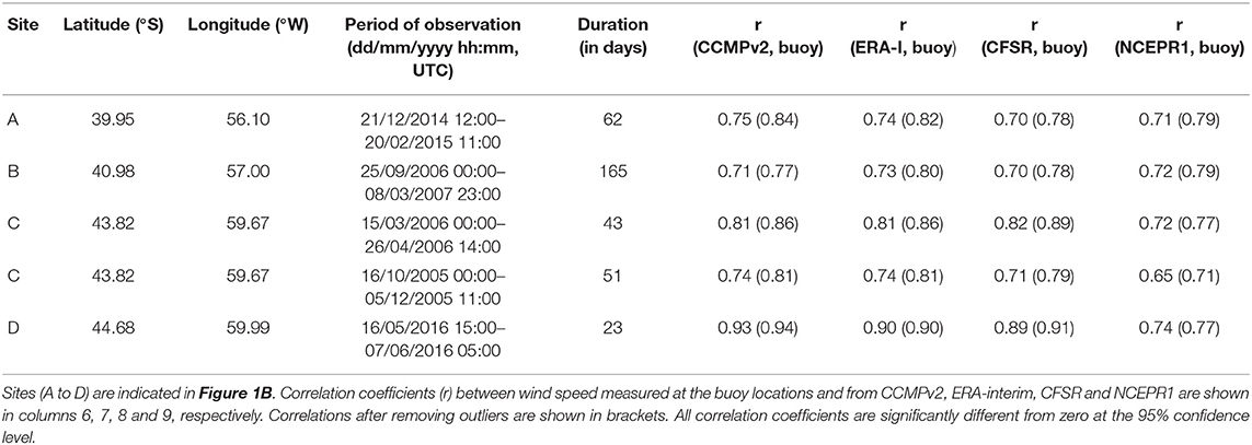
Table 2. Positions, period of observation and duration of the 10 m wind records (columns 1 to 5) from meteorological buoys.
2.3. Construction of SST and Ancillary Time Series and Trends Computation
As our goal is to study regional interannual and long-term trend variability of SST fluctuations on the PS, SST monthly means are calculated at each grid point from the daily fields, as well as the record-length monthly mean climatology produced as the mean values for each month. To obtain the SST anomalies (hereafter SSTa) at each grid point we subtracted the monthly climatological annual cycle calculated for the period between 1982 and 2017 from the monthly SST record. To preserve the variability of SSTa at interannual timescales (3–7 years), we evaluated centered running mean filters by varying the windows length from 12 to 48 months. For this study we selected a 36-month window. Note that similar results are found when a longer window length is considered (not shown). We choose to be conservative and use the 36-month filter in order to lose only 18 months at the beginning and at the end of the record and yet retain most of the interannual variability.
Long-term trends of SSTa are calculated at each grid point over the domain defined by 110°-10°W and 10°-60°S by linear regression of the monthly data with regression coefficients estimated by ordinary least squares, and their significance is tested using Mann Kendall's non-parametric trend test with a 95% confidence level (Mann, 1945; Kendall, 1955; Hirsch et al., 1991; McLeod et al., 1991). The Mann Kendall trend test is a non-parametric test for randomness against the trend and has been extensively applied in meteorology and oceanography. The null hypothesis of randomness states that the data are a sample of n independent and identically distributed random variables. In this study, the number of independent variables of filtered time series was calculated following the methodology of degrees of freedom proposed by Emery and Thomson (2014). From the distribution of SSTa trends, three regions of interest are selected a posteriori on the PS because of their significance, hereafter referred to as Northern Patagonian Shelf (NPS), Central Patagonian Shelf (CPS), Southern Patagonian Shelf (SPS), which will be described in detail shortly (see Figure 1B and Table 3). The SSTa time series are spatially averaged within each region for each monthly time step resulting in three time series that represent the temporal SSTa variability at NPS, CPS, and SPS, respectively. To examine the relationship between local atmospheric forcing and the observed long-term trends and variability of SSTa we analyzed winds and surface heat flux anomalies. For each region, all the above-mentioned variables were monthly averaged and filtered with an 36-month running averaged identical to the SSTa (described above).
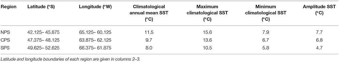
Table 3. Basic statistics of Sea Surface Temperature for the regions NPS, CPS, and SPS.
2.4. EOF Analyses
To determine the dominant spatial and temporal patterns of interannual variability of SSTa, we carried out an empirical orthogonal function (EOF) analysis (Preisendorfer and Mobley, 1988). The EOF is made over the spatial domain over the region 110°-10°W and 10°-60°S, after removing the record-length trend from the records. The temporal evolution of the spatial pattern of each EOF is described by its principal component time series (PC).
3. Results
The results are presented as follows: in Section 3.1 the different wind products are evaluated against the in-situ observations collected with the four moored buoys (black dots in Figure 1B). In Section 3.2 we present the analyses of the linear trends of SSTa in the region of study. Subsequently, we analyze the possible physical drivers of observed SSTa variability at interannual time scales and the possible relationship between SSTa and the local atmospheric forcing on the PS, by evaluating the variability of surface wind, sea level pressure, and sea-air heat fluxes. Section 3.3 presents the analysis of the leading modes of SSTa variability around southern South America and their possible link with large-scale climate indices.
3.1. Performance of Wind Products
Comparisons of climatological wind stress and wind stress curl in the southeast Southeastearn Pacific Ocean (SEP) and SWA estimated from NCEPR1, CFSR, Era-Interim, and CCMPv2 data during the overlapping period (1987–2017) reveal substantial differences in spatial distribution (Figure 2). In general, CCMPv2 wind stress curl shows more complex spatial distribution among the four products, while reanalyses display smoother patterns. This can be noted in the BMC region and around 50°S in the SWA. While the spatial patterns of ERA-Interim and CFSR agree well, there are areas where CFSR presents higher absolute values than ERA-interim. For example, the estimated wind stress curl in the Drake Passage is −0.4x10⁴ N m−2 km−1 ERA-Interim and –0.6 x 10⁴ N m−2 km−1 CFSR. Similarly, in the BMC, the wind stress curl reaches 0.5 x 10⁴ N m−2 km−1 CFSR and 0.2 x 10⁴ N m−2 km−1 ERA-Interim, possibly due to the higher spatial resolution of the latter. Compared with the other datasets, NCEPR1 displays a wider area of negative wind stress curl north of 36°S in the SEP. The wind stress curl is less intense in NCEPR1: in the subtropics the maximum values are 0.3x10⁴ N m−2 km−1 in NCEPR1 and larger than 0.5x10⁴ N m−2 km−1 in CCMPv2, ERA-Interim, and CFSR.
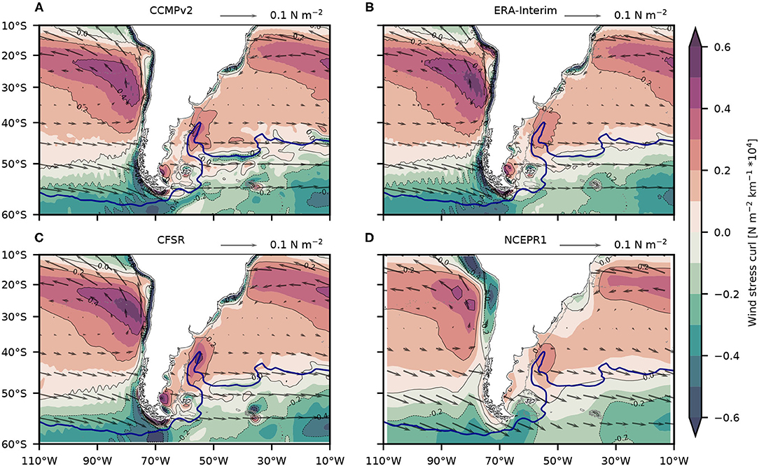
Figure 2. Distribution of climatological wind stress at 10 m height (vectors) and wind stress curl (background shading) during 1988–2017 from (A) CCMPv2, (B) Era-Interim, (C) CFSR, and (D) NCEPR1. Wind data are described in Section 2.2. Positive wind stress curl indicates anticyclonic wind stress circulation and negative wind stress curl indicates cyclonic circulation. Vectors are shown every 20 gridpoints for CCMPv2 and ERA-Interim, every 10 gridpoints for CFSR and every 3 gridpoints for NCEPR1. The solid dark blue line represents the mean location of the Subantarctic Front (SAF, Kim and Orsi, 2014).
There are notable regional differences among the four wind databases analyzed here. To further investigate these differences on the PS, we compared time series of wind speed of atmospheric reanalysis (NCEPR1, CFSR and ERA-Interim) with CCMPv2 to determine which is the most suitable dataset for the region. We estimate the correlation coefficients (r) and root-mean-square error (RMSE) between wind speed for filtered and non-filtered time series at NPS, CPS, and SPS. The statistical significance of the correlation coefficients is calculated evaluating the degrees of freedom of each time series (Thomson and Emery, 2014) and are listed in Table 4. The highest correlation and the smallest RMSE are obtained between ERA-Interim and CCMPv2. This comparison is helpful as we wish to identify the most accurate reanalysis to analyze the atmospheric surface forcing in the study region. The correlation coefficients of the 36-month filtered wind data are higher than for non-filtered monthly records. For example, the correlation coefficients of wind speed at NPS between CCMPv2 and ERA-Interim are 0.66 and 0.86 for non-filtered and filtered data, respectively, indicating that the discrepancy between the two products increases at higher frequencies. Consistently, this is also noted in the smaller RMSE for filtered records. The correlation coefficients between ERA-Interim and CFSR (both filtered and non-filtered records) are statistically different from zero at 5% error probability. However, the highest correlations are found between CCMPv2 and ERA-Interim after 36-month low pass filtering, indicating that the latter is a suitable reanalysis to use for evaluating the atmosphere-ocean interactions on the PS. The reader is reminded that CCMPv2 uses ERA-Interim reanalysis as the first-guess wind field and therefore the data are not entirely independent from each other.
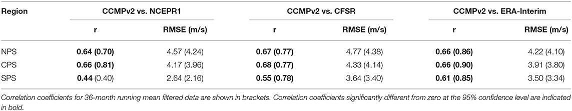
Table 4. Linear correlation coefficients (r) and root-mean-square error (RMSE) of 10 m wind speed derived from CCMPv2 and from reanalysis NCEPR1, CFSR and ERA-Interim at NPS, CPS and SPS.
Winds in the open ocean are notoriously difficult to validate, and there are limited in-situ data to match the location and time of reanalyses and other wind products. Based on the above-mentioned results, in Figure 3 we present a comparison between ERA-Interim, CCMPv2 and the longest in-situ wind data available in the SWA shelf break at 40.98°S, 57°W. The in-situ observations extend from 25 September 2006 to 8 March 2007 (Site B, Figure 1 and Table 2). The hourly buoy data were sub-sampled to match the 6-h winds at 10 m (00, 06, 12, and 18 UTC) from ERA-Interim and CCMPv2. Note that wind speed is referenced at 10 m height in CCMPv2 and ERA-Interim, while buoy winds were observed at 4 m height. We adjusted the 4 m in-situ wind speed observations to 10 m height following Atlas et al. (2011). This adjustment leads to a 13% increase in time-mean wind speed compared to the original 4 m winds. The correlation coefficient between adjusted in-situ wind speed and CCMPv2 (ERA-Interim) is 0.71 (0.73). Removing outliers, defined as values above and below ± 2 standard deviations (SD), the correlation improves to ~0.80 for CCMPv2 and ERA-Interim. Correlations with and without outliers are statistically significant at 5% error probability. The linear least-square adjustment between in-situ and CCMPv2 data indicates that at this location the scatterometer-derived winds tend to overestimate buoy observations at wind speeds lower than 5 m s−1, and underestimate it at higher wind speeds. Similar results are found for ERA-Interim reanalysis, though the transition occurs at a higher wind speed (8.5 m s−1, Figures 3C,D). The correlation coefficients for the other deployments (Sites A, C and D, Figure 1) are listed in Table 2. The best adjustment is found at Site D, possibly because the wind speed was less variable at that site during the time of deployment. Correlation coefficients between ERA-Interim/CCMPv2 and in-situ wind speed observations at the four locations range between 0.71 and 0.93, indicating a relatively good adjustment with ERA-Interim/CCMPv2 wind speed. Given the similar performance of both datasets and that CCMPv2 products are available only since early 1987, in the following analyses we use ERA-Interim reanalysis which also provides consistent surface heat-flux estimates and covers the same time period as the SST observations analyzed here. The same comparison was made between in-situ wind data and CFSR / NCEPR1 reanalysis obtaining a lower correlation compared with the correlation with ERA-Interim / CCMPv2, except for one measurement point (Site C, Period of observation 15/03/2006 00:00–26/04/2006 14:00) where the correlation coefficients with CFSR are slightly higher (Table 2).
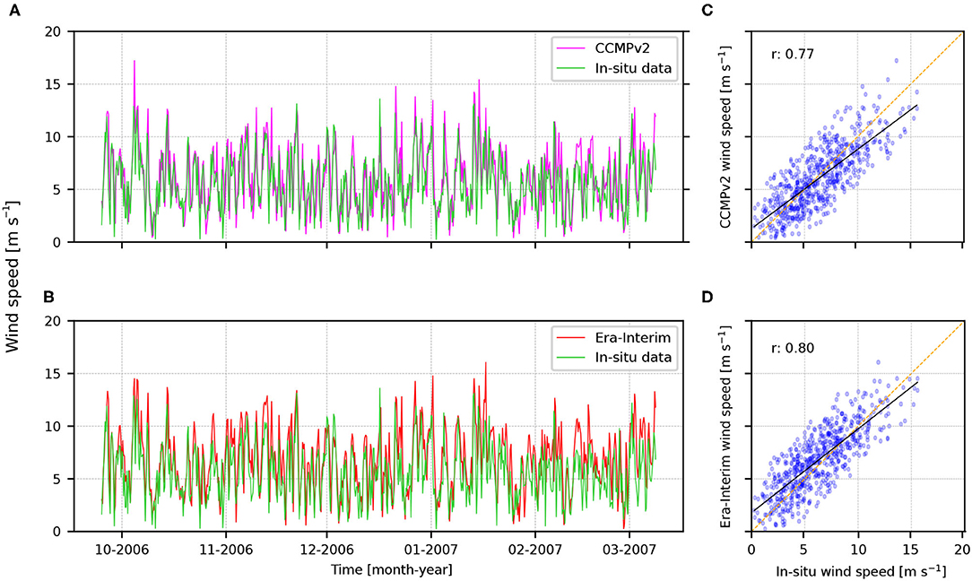
Figure 3. Comparison of wind speed time series from: hourly in-situ data (solid green line) from an oceanographic buoy located at 40.98°S, 57°W (Site B, Figure 1B and Table 2) and (A) CCMPv2 (solid magenta line) and (B) Era-Interim (solid red line) data extracted at the nearest grid point. The wind speed data from CCMPv2 and Era-Interim used here have a 6-h temporal resolution. (C,D) Scatter plot between the time series shown in (A,B) together with the linear fit by least-squares (solid black line). r is the correlation coefficient and the line y = x is shown in orange.
3.2. Linear Trends and Temporal Variability of SSTa
3.2.1. Spatial Distribution of SSTa Linear Trends Between 1982 and 2017
The spatial distribution of record-length satellite-derived linear trends of 36-month filtered SSTa (Section 2.1) in the SEP and SWA is shown in Figure 4 (only significant trends at the 95% confidence level are shown). The distribution of SSTa trends reflects large-scale patterns. The largest positive and negative trends are observed along the BC and the BMC (around 0.4°C decade−1) and in the central Drake Passage (< −0.3°C decade−1), respectively. Significant warming (positive) trends are located in mid-latitudes between 20 and 50°S. Most of these areas in the SWA are located north of the Subantarctic Front (SAF, green line in Figure 4, extracted from Kim and Orsi, 2014), suggesting that the majority of the warming occurs within the South Atlantic Subtropical Gyre (i.e., north of the SAF). In particular, the SWA region has been identified as a warming hotspot where SST is increasing faster compared to other regions (Hobday and Pecl, 2014; Hobday et al., 2016) and recent analyses from satellite data and models suggest that the warming is associated with a southward migration of the South Atlantic subtropical gyre and a southward penetration of the Brazil Current (e.g., Yang et al., 2020; Goyal et al., 2021). Notably, the shallow (<10 m) inner region of Rio de La Plata estuary registers the largest positive linear trend (> 0.8 °C decade−1). In contrast, cooling (negative) trends are found north of 25°S and south of 50°S, except for the region east of 45°W that presents moderate warming. The most intense cooling in this domain is located in the western Scotia Sea and Drake Passage (centered around 56°S–60°W). Only about 20% of the grid points in the full domain present cooling trends. Along the path of the MC, linear trends are slightly negative but mostly non-significant, except for a small region close to its northernmost extension near 39°S (< –0.2°C decade−1). The large-scale meridional dipole pattern of linear trend distribution in the SWA extends over the PS, with positive trends north of 46°S, neutral trends around 48°S, and negative trends south of 49°S. Motivated by the potential impacts of SSTa variability on the productive Atlantic Patagonian Shelf, we will focus our subsequent analyses on SSTa time series constructed at the selected regions (NPS, CPS and SPS; Figure 5; Section 2.3). NPS and SPS are located at the positive (northern) and negative (southern) sides of the above-described dipole of meridional SSTa trends, respectively, while CPS is located in the neutral transition zone (see regions indicated in Figure 4), where no significant trend is observed. At NPS and SPS, the magnitude of warming and cooling trends is similar: 0.15 ± 0.01 and –0.12 ± 0.01 °C decade−1, respectively. For the entire period spanning between 1982 and 2017, these linear trends represent variations of almost half a degree, with an increase of 0.52°C at NPS and a decrease of –0.42°C at SPS.
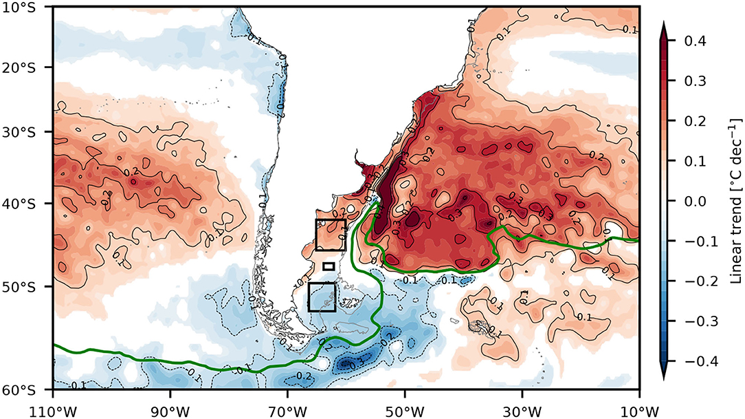
Figure 4. Observational trends of filtered SST anomalies (SSTa) for the 1982–2017 period. SSTa are obtained by subtracting the climatological annual cycle calculated for the same time period from the SST record at each grid point and then smoothed by a 36-month running mean (see Section 2.1). Only regions where trends are significant at a 95% confidence level (after Mann Kendall's-test) are shaded. Black rectangles indicate the NPS, CPS, and SPS regions (identical to the boxes in Figure 1B). The solid dark green line represents the mean location of the Subantarctic Front (SAF, Kim and Orsi, 2014).
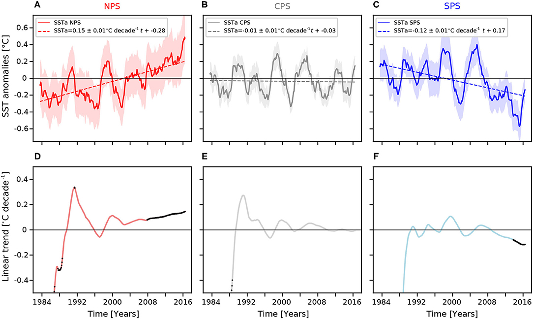
Figure 5. (Top) Time series of 36-month running mean of SSTa (solid line), standard deviation (shaded) and linear trend fit (dashed line), together with their corresponding linear trends based on the SST data set described in Section 2.1 at (A) NPS (B), CPS, and (C) SPS shown in Figure 1B. The construction of the SSTa time series for each regions is described in Section 2.3. Trends at NPS and SPS are significant at the 95% confidence level. (Bottom) Temporal evolution of linear trend slope between 1982 and 2017, at (D) NPS, (E) CPS, and (F) SPS. Values for the time steps when the linear trends are significant at 95% confidence level are marked in black.
The PS presents a large amplitude seasonal cycle of SST, with mean amplitudes exceeding 5°C over most of the domain (Rivas, 1994, 2010). It is therefore relevant to determine to what extent the long-term trends are associated with specific seasons. To this end we analyzed the seasonal linear trends of SSTa (Supplementary Figure S1). Seasonal trends of non-filtered SSTa present warming in mid-latitudes of SEP and SWA that are larger in February and March (late austral summer) and exceed 0.3°C decade−1 at NPS. These positive trends remain significant but are weaker (0.2–0.3°C decade−1) during April and May (austral autumn) and July and August (austral winter). The cooling signal is stronger (< –0.2°C decade−1) at SPS during January and February (austral summer), indicating that summers have become colder over the period of observation analyzed here. A possible driver of the observed cooling could be enhanced vertical mixing within the upper water column. In the remaining of the year, there is no significant trend on the PS.
3.2.2. Interannual Variability of SSTa on the PS Between 1982 and 2017
The focus of this section is to study the interannual variability and the temporal evolution of SSTa linear trends in the PS. We examine the frequency distribution of the variability in the detrended time series of SSTa at NPS, CPS and SPS based on the variance preserving power spectral density of filtered and detrended time series using the Welch method (Welch, 1967; Figure 6). The data were divided into five 16-year segments with 75% overlap. A Hamming window was used to compute the modified periodogram of each segment. At interannual time scales, the spectra of the three records present a significant peak centered at about 80 months (~6 years) reaching maximum SSTa variance at SPS (0.032 °C2) and minimum SSTa variance at NPS (0.02 °C2). In both cases ~70% of the total variance is associated with the frequency band between 3 and 10 years. Spectral variance at periods shorter than 36 months is effectively removed by the running means.
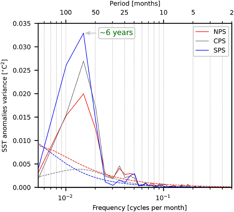
Figure 6. Variance preserving Welch spectra of filtered and detrended SSTa time series (see Section 2.1) at NPS (solid red line), CPS (solid gray line) and SPS (solid blue line) shown in Figure 1B). Dashed lines indicate the power spectral density of red noise for each spectrum. The dashed green line indicates the period of maximum variance centered at ~6 years (see Section 3.2.2).
The SSTa time series at NPS and SPS present similar interannual fluctuations displaying large positive anomalies centered in 1990, late 1998, and 2005, and sharp negative anomalies in 1996 and late 2001 (Figure 7A). To address the similarities and differences in the temporal evolution of SSTa at NPS and SPS, we computed the time series of the correlation coefficient between both variables (Figure 7B). The linear correlation is positive and significant until ~2010. After 2008 the correlation decreases and becomes progressively negative, though it does not exceed the 95% confidence level at the end of the record. Since the attribution of linear trends depends on the end-points of the time series, we define the year 2008 as a “breakpoint” and analyze the 1982–2007 and 2008–2017 periods separately instead of the entire record. Before 2008, there are no significant linear trends of SSTa at either of the three selected regions on the PS. In contrast, during 2008–2017, significant positive linear trends are observed at NPS: 0.35 ± 0.02°C decade−1, at SPS –0.27 ± 0.03°C decade−1, while at CPS there is no significant trend. Thus, the record-length SSTa trends observed at NPS and SPS are mostly associated with the variability observed during the last 10 years of the records.
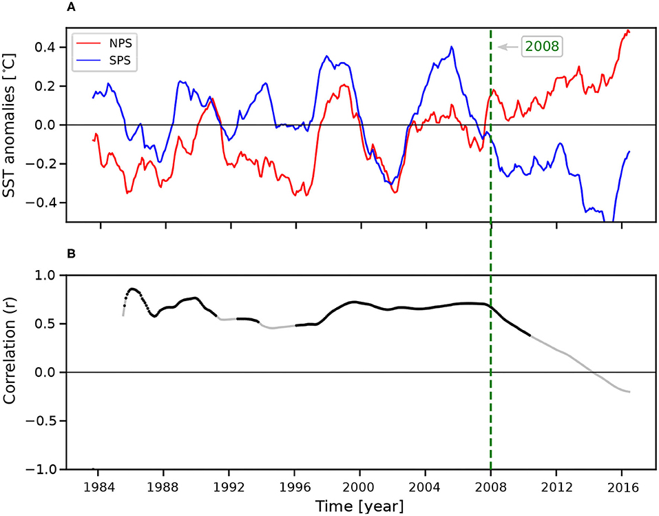
Figure 7. (A) Time series of filtered SSTa at NPS (solid red line) and SPS (solid blue line). The time series are identical to those shown in Figures 5A,C. (B) Temporal evolution of the correlation coefficient (r) between SSTa at NPS and SPS. Heavy black lines indicate significant correlations at the 95% confidence level. The dashed green line indicates the “breakpoint” year centered at 2008 as identified in Section 3.2.2.
3.2.3. Physical Drivers of Observed SSTa Trends Variability on the PS
Due to the behavior shift of the SSTa prior to and after 2008 on the PS (Figure 7), the spatial distribution of linear trends is analyzed over the SEP and SWA dividing the full-length record in two periods: 1982–2007 and 2008–2017. As mentioned earlier, large interannual variations of SSTa are observed on the PS (Figure 6). The interannual variability will be analyzed in detail in Section 4.3. To investigate the possible role of physical drivers on the observed linear SSTa trends over the SEP and SWA prior to 2007 and after 2008, we examined the relationship between the SSTa and the anomalies of the zonal and meridional wind components (u-wnda and v-wnda, respectively), wind speed (wspda), wind stress curl (curla), sea level pressure (SLPa), and net surface heat-flux (nhfa) from ERA-Interim (see Section 4.1). Subsequently, we compared SSTa with the above-mentioned atmospheric anomalies during 1982–2007, 2008–2017, and 1982–2017 (full record) at NPS, CPS, and SPS. Linear correlation coefficients between SSTa and atmospheric variables are listed in Table 5 with significant values (95% confidence) indicated in bold. The correlation coefficients between all heat flux components (long and short-wave radiation, latent and sensible heat) and SSTa are low and non-significant (not shown). Thus, only the net heat flux is presented in Table 5.
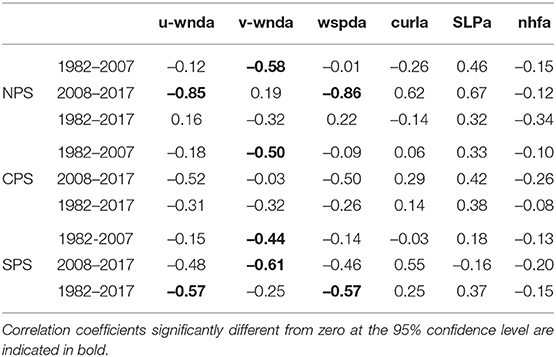
Table 5. Linear correlation coefficients (r) between the time series of atmospheric forcing and SSTa at NPS, CPS, and SPS for different time periods: between 1982 and 2007, between 2008 and 2017, and for the full records between 1982 and 2017 (see Section 4.2.2).
3.2.3.1. Linear Trends During 1982–2007
The spatial distribution of linear trends of SSTa for the period 1982-2007 exhibits moderate warming trends in the SWA (~0.2°C decade−1), located over the Zapiola gyre (centered roughly at 44°S, 45°W) and south of 20°S along the main path of the BC (Figure 8A), while trends over the continental shelf are mostly neutral, except for the inner Río de la Plata and the South Brazil Bight. Over the SEP, significant warming greater than 0.2°C decade−1 is observed between 24 and 40°S and west of 90°W, which is also apparent in the SSTa trend distribution for the entire 1982–2017 period (see Figure 4). During 1982–2007, only weak cooling trends are observed mostly located south of 50°S.
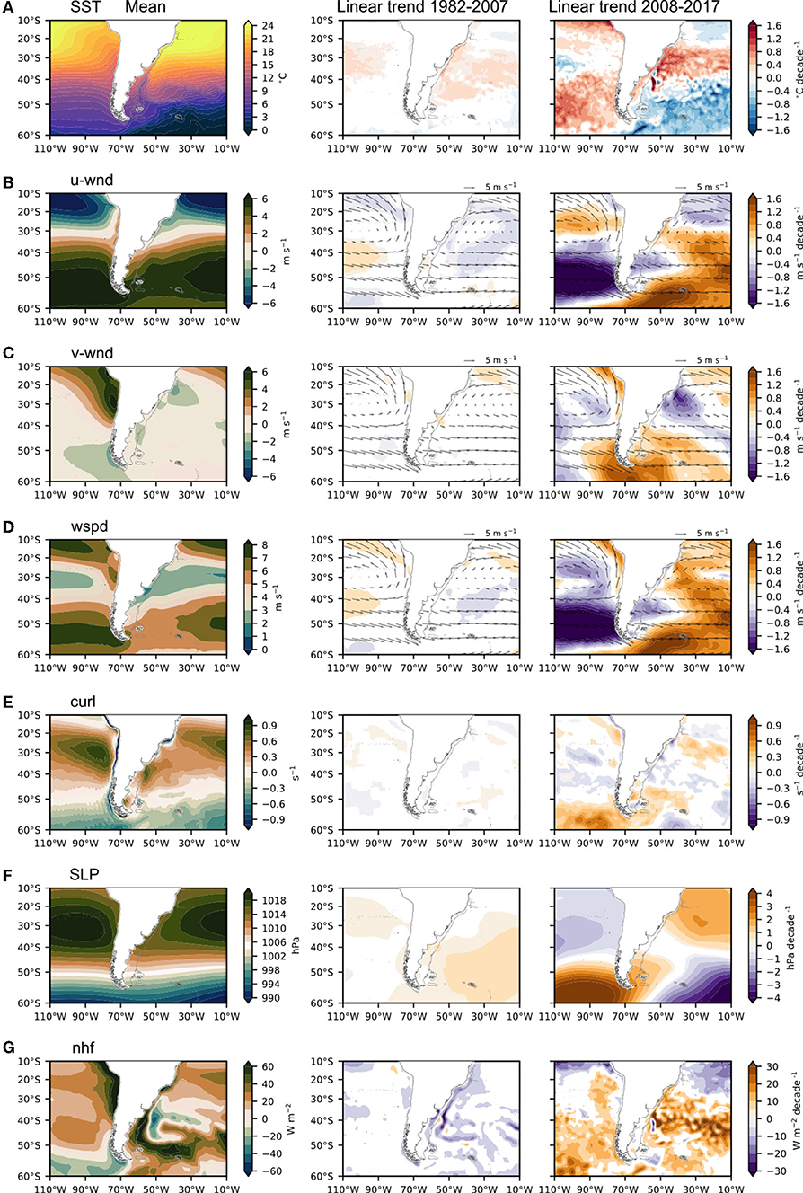
Figure 8. (Left) Distribution of climatological (A) SST, (B) u-wnd, (C) v-wnd, (D) wind speed, (E) wind stress curl, (F) SLP, and (G) net heat flux for the 1982–2017 period. The wind speed, SLP and heat flux data are from Era-Interim (see Section 2.2). The spatial distribution of the linear trends of filtered anomalies of each variable are shown in the left panels (see Section 2.3 for methodology) calculated over 1982–2007 (center) and 2008–2017 period (right) (see details of selection of time periods in Section 3.2.2). Vectors in (B–D) show the distribution of climatological wind speed at 10 m height during 1982–2007 (center) and 2008–2017 (right) periods. Vectors are shown every 20 gridpoints. In every panel the 200 m isobath is also shown (solid gray line).
The zonal wind component u-wnda in the SWA presents a negative trend (–0.4 m s−1 decade−1) north of 50°S and a positive trend over a few small regions further south, with a magnitude ranging between 0.2 and 0.4 m s−1 decade−1 (Figure 8B). This distribution is consistent with the positive SLPa trend of around 1 hPa decade−1 centered near 50°S, 30°W which leads to weaker westerlies between 30 and 50°S and stronger westerlies south of 50°S (Figure 8F). U-wnda trends over the continental shelf are slightly positive (0.2 m s−1 decade−1) between 40 and 50°S and negative off the Rio de la Plata. Over the SEP, positive u-wnda trends are located in mid-latitudes between 35 and 50°S, and negative north of 20°S (intensified trades) and south of 55°S (weakened westerlies). Trends in the meridional wind, v-wnda, are weak or non-significant throughout most of the domain (Figure 8C). Thus, the linear trend in wind speed distribution follows the spatial pattern of u-wnda trends (Figure 8D). Weak and mostly non-significant trends of curla are found during this period (Figure 8E). The distribution of nhfa trend is mostly neutral or negative over the SWA (-8 W m−2 decade−1), particularly along the path of the BC, and over the outer continental shelf north of 50°S, where it exceeds –10 W m−2 decade−1, and the Rio de la Plata estuary. This indicates a larger heat loss from the ocean in the southern portion of the BC and the BMC. In contrast, the estimated trend suggests a weaker heat gain in shelf break region north of 50°S (Figure 8G). In the SEP negative nhfa trends are observed near 10°S 100°W.
To summarize, during the 1982-2007 period the continental shelf between 35 and 55°S presents non-significant SSTa trends. The region is dominated by weak and positive u-wnda trends resulting in stronger eastward wind speed. Non-significant or very weak trends are observed in v-wnda, curla, and SLPa. There is a significant negative trend of nhfa at northern PS, on average of –8 W m−2 decade−1. In conclusion, though the interannual variations remain important during this period (see Section 4.4) weak trends are observed on the PS in the wind components, wind-derived fields and the SSTa linear trend distribution.
Over the 1982–2007 period, significant negative correlations are found between SSTa and v-wnda at NPS, CPS, and SPS (r = –0.58, –0.50, and –0.44, respectively, Table 5). During this period, there is no linear trend of SSTa at the three selected regions of the PS, indicating that the observed fluctuations are, at least partially, dominated by interannual variability. The significant relationship between SSTa and v-wnda suggests that part of the SSTa variability is modulated by meridional wind variability. These fluctuations of meridional wind intensity may drive the temperature changes reported here by inducing changes in the northward advection of cold waters through the southern boundary of the continental shelf. This process will be further discussed in the next section. In contrast, there is no significant correlation between SSTa and the other variables analyzed here (Table 5).
3.2.3.2. Linear Trends During 2008–2017
The spatial distribution of linear trends of SSTa during 2008–2017 feature notable differences in magnitude and spatial patterns relative to the 1982–2007 period. While in 1982–2007 the SSTa trends as well as the trends of the analyzed forcing terms are null or weak (Section 4.2.3.1, center panel in Figure 8A), in the most recent period since 2008 the trends become stronger and significant (Figure 8A). Thus, this spatial pattern resembles the pattern of the full record length trends (Section 4.2.1), but the trends are now more intense. As in Figure 4, in the SWA significant warming trends (> 0.5°C decade−1) extend over the South Atlantic subtropical gyre and the continental shelf between 25 and 40–45°S, reaching maximum values in the BMC (> 1.5°C decade−1) and in the Rio de la Plata estuary (> 0.8°C decade−1) (right panel in Figure 8A). Cooling areas in the SWA are mostly located south of 40°S in the open ocean and extend over an outer portion of the southern PS. The largest negative trends are observed in the central Drake Passage and extend eastward up to 50°W with values exceeding -1.0°C decade−1. The eastern SEP presents sharp warming trends between 10–20°S and between 35–60°S, ranging from 0.2 to 1°C decade−1, while in the western SEP moderate cooling extends between 30 and 35°S.
Over the SEP, positive trends of u-wnda are located in the subtropics between 15 and 35°S (i.e., weakened trades) and negative south of 35°S (i.e., weakened westerlies, Figure 8B). This is consistent with weakened meridional gradients of SLP suggested by the distribution of SLPa (right panel in Figure 8F). In the SWA south of 48°S there is a significant increase of u-wnda (reaching maximum values of about 1.2 m s−1 decade−1 in the Drake Passage, right panel in Figure 8B), which is consistent with the strong trends in the meridional gradient of SLPa (right panel in Figure 8F) at that location. The significant intensification of the westerlies could be partially responsible for the observed cooling in this region due to increased northward Ekman transport that advects cooler waters in the upper layer, and enhances the vertical mixing. In tropical latitudes in the SWA, u-wnda trends contribute to enhance easterlies north of 20°S and westerlies further south and east of 30°W by as much as 0.4 to 1 m s−1 decade−1 (right panels in Figures 8B,D). These changes of the lower atmospheric circulation are largely associated with the enhanced meridional SLP gradients (positive SLPa trend of ~2.0 hPa dec-1) centered near 15°S, 25°W and negative SLPa trend further south (right panel in Figure 8F). On the continental shelf and adjacent deep ocean, negative u-wnda trends (–0.6 m s−1 decade−1) are observed between 40 and 50°S and west of 45°W, which lead to weaker westerlies (right panel in Figure 8B). The negative trend in u-wnda leads to a similar trend in wspda (right panel in Figure 8D), which may contribute to the positive SSTa due to decreased wind mixing and increased vertical stratification. The distribution of v-wnda trends in the SWA basin are significant and negative between 18–40°S and 50–30°W (values of –1.4 m s−1 decade−1) leading to increased northerly winds in this region. The trends of v-wnda are positive south of 50°S, with the highest values localized in the western Scotia Sea (1.2–1.6 m s−1 decade−1), resulting in a meridional wind reversal (from northerly to southerly) and continuing increased southerly winds during this period. V-wnda trends are positive over most of the west coast of South America, leading to increased southerly winds north of 30°S. South of 45°S, southerly wind anomalies imply a meridional wind reversal from northerly to southerly (right panel, Figure 8C). V-wnda time series around southern South America indicates that during 2014 and 2015 in-phase southerly wind anomalies prevail on the Pacific and Atlantic shelves (not shown). The trend distribution of wspd-a is highly dominated by u-wnda in the entire domain (Figure 8D). At high latitudes, the trend of curla intensifies over the southern SEP (50°-60°S) and slightly further north over the southwestern portion of the SWA (45°-55°S) with a range of 0.4 to 1 x 10⁴ s−1 decade−1 (right panel in Figure 8E). Negative trends of curla are located south of 54°S and east of 50°W in the SWA (~ −0.5 x 10⁴ s−1 decade−1). These negative wind stress curl trends over regions of negative curl can drive stronger Ekman–induced upwelling and thereby lead to negative SSTa. At low latitudes, north of 20°S in the SEP and north of 30°S in the SWA, there is a significant negative trend of nhfa exceeding –24 W m−2 decade−1 (Figure 8G). In the mid to high latitudes the distribution of nhfa trends is mostly positive, with some regional maxima observed in the BMC (>30 W m−2 decade−1) and in the central Drake Passage (~25 W m−2 decade−1). The localized yet intense nhfa trend dipole pattern observed over the BMC replicates the SSTa pattern, though with opposite signs (i.e., warming regions are associated with negative nhf trends and viceversa). This pattern clearly indicates that SSTa trends are not due to trends in nhfa. Since the region of warm waters north of the BMC is characterized by intense net heat loss to the atmosphere, the negative nhfa trend is consistent with a southward displacement of warm waters, and the associated positive SSTa trend along the narrow meridional strip located near 54°W between 38 and 44°S. Moreover, it suggests a strong modulation of the trends observed in the surface heat flux components by the local SSTa trends, but unraveling the dynamics of this feature is beyond the scope of this paper. Similarly, negative SSTa trends observed south of 40°S in the SWA occur with positive nhfa trends, suggesting that cooling in this region is not a direct response to sea-air heat flux trends.
The meridional dipole of SSTa trends observed on the PS during the entire record (Figure 4, Section 4.2.1) is similar to the one observed in 2008–2017 (right panel in Figure 8A), with values reaching 1°C decade−1 in the northern region and −0.8°C decade−1 in the southern region. Thus, the 2008–2017 SSTa trends shape the trends observed in the full-record, as also observed from the temporal evolution of the SSTa trends at NPS and SPS (Figures 5, 7). The distribution of u-wnda displays negative trends (decreased westerlies) and the v-wnda trends (0.4–0.8 m s−1 decade−1, right panel in Figure 8C) indicate southerly wind anomalies that reverse the meridional wind from northerly to southerly approximately in 2012 (not shown). These changes in surface wind imply an anticyclonic circulation anomaly which leads to the positive trend of curla observed between 40 and 51°S on the PS (right panel in Figure 8E). This pattern drives an anomalous convergence of surface water that could enhance the positive SSTa trend observed at NPS in 2008-2017. However, this mechanism cannot explain the negative trend of SSTa observed at SPS. At the eastern mouth of the Magellan Strait (52°S), there is a region of negative curla trend, which acts to weaken the downwelling associated with the positive record-length mean curl (left panel in Figure 8E). Positive SLPa trends observed on the PS south of 45°S result in strong negative trends in u-wnda north of 50°S and positive trends further south. Significant linear correlations between u-wnda (and wspda) and SSTa are found at NPS (r = –0.85 and –0.86, respectively). This indicates that the positive trend of SSTa observed in this region is associated with a decrease in the local zonal winds. At SPS, there is a significant correlation between SSTa and v-wnda (r = –0.61), indicating that the decreasing SSTa occurs partially in response to the above described reversal in meridional wind, by enhancing the northward advection of relatively cold waters. Numerical simulations suggest that the interannual variations of along-shelf transport in the southern portions of the continental shelf are moderately modulated by the meridional wind stress variability, which sets-up a cross-shelf pressure gradient through Ekman dynamics and thus geostrophically drive along-shelf transport variations (Combes and Matano, 2018; Guihou et al., 2020). Moreover, the interannual fluctuations of meridional wind are closely associated with SAM. Some small areas of significant negative nhfa trends are observed in the inner PS, while in the remaining of the PS the nhfa trends are non-significant (right panel in Figure 8G). At the northern PS, the negative rate of nhfa does not seem to be associated with the positive SSTa trends, indicating that heat fluxes are not responsible for the observed warming at these timescales.
During the entire period (1982–2017), significant negative correlations are found at SPS between SSTa and u-wnda (r = –0.57), and wspda (r = –0.57). These negative correlations suggest that the decreased SSTa is partially a response to enhanced vertical mixing associated with the increased u-wnda that are more intense during 2008–2017. The correlation coefficients between the SSTa and the other atmospheric variables considered (v-wnda, curla, SLPa, and nhfa) are not significant in all regions analyzed (Table 5).
3.3. Leading Modes of Interannual SSTa Variability
To further investigate the nature of the interannual variability which dominates the SSTa around southern South America at periods of nearly 6 years (Figures 5, 6) we carry out an EOF analysis of detrended SSTa in the domain bounded by 110°-10°W, 10°-60°S. Figure 9 depicts the leading modes of filtered SSTa during the entire record (1982–2017). Each EOF pattern is multiplied by the square root of their eigenvalues so that the amplitude of each mode is scaled in °C. The first mode (EOF1, left panel in Figure 9A) explains 28% of the total SSTa variance and resembles the first mode of SSTa variability documented by previous studies for different time periods (Deser et al., 2010; Messié and Chavez, 2011). This mode exhibits negative SSTa near the tropics associated with a characteristic ‘horse-shoe shaped’ pattern present on the tropical Pacific that usually extends along the west coast of North and South America. EOF1 presents maximum variance over the subtropics of the eastern South Pacific and over the subpolar South Atlantic east of 30°W. The second mode (EOF2, left panel in Figure 9B), which accounts for 16% of the total SSTa variance, displays most of the variance centered in the SWA with an out-of-phase relationship between SSTa north and south of about ~40°S. This dipole pattern extends on the PS, though with weaker amplitudes (< |0.1|°C) suggesting a possible linkage between the shelf SSTa variability and a basin-scale pattern of variability. The maximum values in the southern center of action are located close to the SAF, where SSTa ranges between 0.2 and 0.3°C. EOF3 (right panel in Figure 9C) explains 12% of the variance with maximum positive values located close to BMC and negative values north of 20°S. Thus, the combined three leading modes explain 56% of the variance of filtered SSTa. Similar results are obtained applying running means considering shorter time windows to compute the filters: 55% of the total variance is explained by the first three modes when 24-months filter is used and the total variance explained is only slightly higher (57%) when 18-months filter is used (not shown). The variance explained by the three leading modes of non-filtered monthly SSTa decreases to 31%, suggesting that the importance of the most significant modes increases for longer time scales.
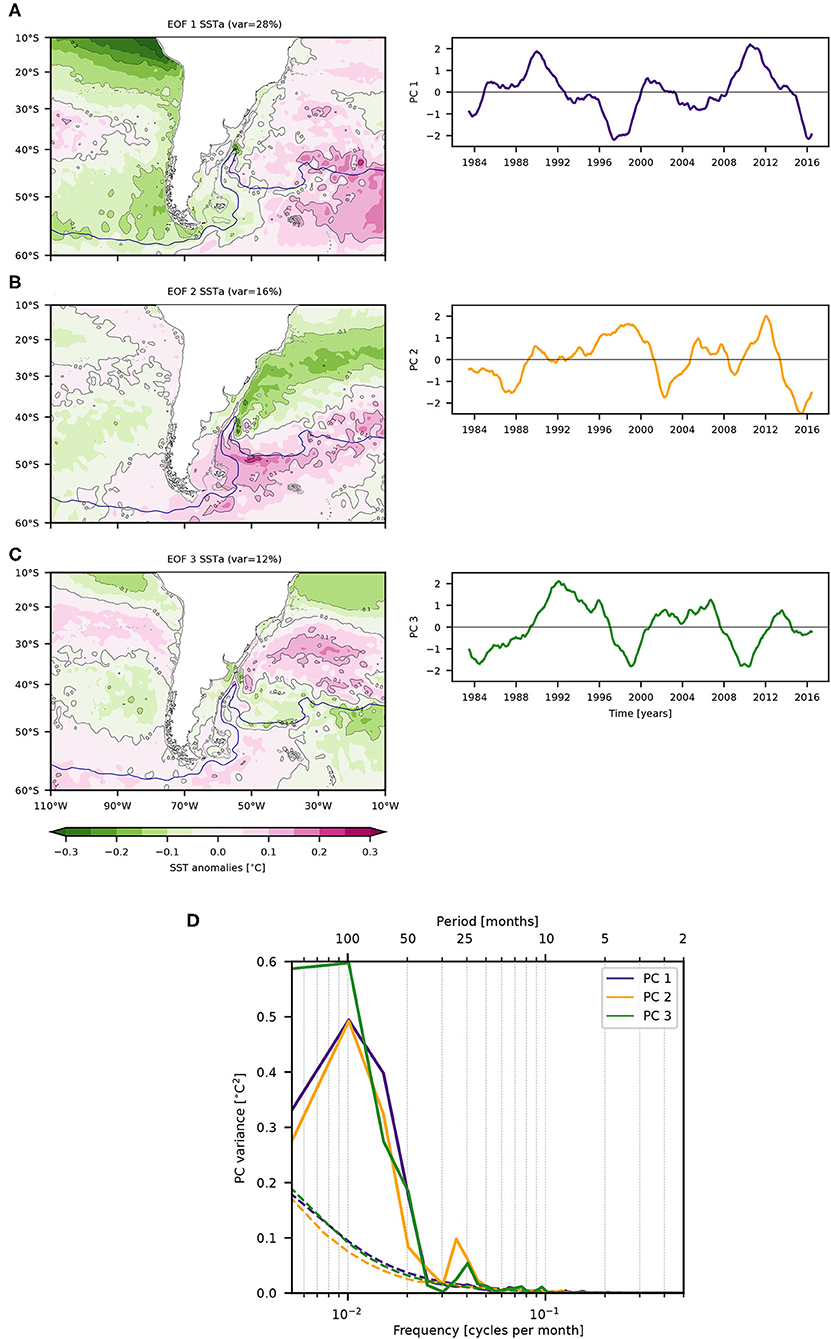
Figure 9. (Left) First three (A–C) leading EOF of filtered and detrended SSTa estimated over the period 1982–2017 (Section 3.3) and (right) Principal Components (PC) time series of each EOF in normalized units (see Section 2.4 for methodology). The solid gray line in the EOF indicates the 200 m isobath and the solid dark blue line indicates the mean location of SAF (identical to Figures 2, 4). (D) Variance preserving Welch spectrum of the corresponding PC time series for the three leading EOF (solid violet, orange and green lines, respectively). The power spectral density of red noise for each spectrum is indicated by the dashed lines (see Section 3.3).
To investigate the sensitivity of the EOF to the selected spatial domain, we repeated the analysis after dividing the region into two subregions: SEP (110°-70°W, 10°-60°S) and SWA (70°-10°W, 10°-60°S) (not shown). The spatial pattern of EOF1 in SEP is nearly identical to the pattern displayed in the Pacific sector of EOF1 of the entire domain and their corresponding PC time series are almost perfectly correlated (r = 0.97). The spatial pattern of the Atlantic sector of EOF2 from the entire domain is similar to EOF1 of the SWA domain and the correlation between their PC time series is very high (r = 0.99). For the third mode, the correlation between PC3 of the entire domain and PC3 over the SWA is significant and negative (r = –0.75), and positive but non-significant with PC3 of SEP (r = 0.51). This analysis indicates that EOF1 and EOF2 of the entire domain (Figure 9) are associated with modes of SSTa variability centered over the SEP and SWA basins, respectively; while EOF3 combines variance from both basins. We also carried out an EOF analysis of SSTa over the continental shelf domain. The first mode, which explains 38% of the variance, resembles EOF2 of the entire domain. The second mode accounts for 16% of the total SSTa variance. This further illustrates the strong link between the western South Atlantic SST and the variability over the continental shelf at interannual time scales. In the remaining of this paper, we will only use the spatial patterns and PC time series that correspond to the full domain (right panels in Figure 9). The variance preserving spectra of PC1 has its most energetic fluctuations at interannual to decadal timescales (4–12 years) with a peak in spectral variance in periods of about 120 months (10 years) that accounts for ~50% of the total variance (Figure 9D). The PC2 spectrum presents a similar peak, while PC3 presents spectral density accumulated in the band of 4–16 years that accounts for ~70% of the total variance, with higher variance in comparison with PC1 and PC2. The sum of PC1 and PC2 is significantly correlated with the detrended SSTa at SPS (r = 0.71), accounting for 51% of the variance explained by these two principal components. The correlation with detrended SSTa at NPS is very low and non-significant (r = 0.1).
The observed fluctuations of SSTa on the PS are partly associated with the variability of the three previously described leading EOF modes. Thus, we will explore the relationship between the temporal evolution of the PCs and large-scale patterns of the climate system that could drive the interannual SSTa variability by atmospheric and/or oceanic teleconnections. We focus the discussion on three main patterns of variability that are known to impact on extratropical ocean basins in the southern hemisphere on interannual to decadal timescales: Southern Annular Mode (SAM), El Niño Southern Oscillation (ENSO) and the Interdecadal Pacific Oscillation (IPO). The SAM index measures the strength of the meridional pressure gradient around Antarctica (Thompson and Wallace, 2000). The increasing trend to a positive SAM index observed during the past decades has led to the intensification and poleward shift of the westerly winds (Hall and Visbeck, 2002) affecting the local atmospheric forcing on the PS and therefore the response on the SST in that region. On the other hand, the interannual variability of tropical Pacific SST depicted by ENSO events (periods of positive ENSO 3.4 index) can trigger atmospheric Rossby waves that propagate poleward and eastward, modulating regional changes of SST in the southern SWA by local changes on zonal and meridional surface winds (Turner, 2004; Meredith et al., 2008). In addition, we include the IPO in the analysis, a broader SST pattern associated with Pacific-wide SSTs (Henley et al., 2015) on interdecadal timescales. Recent studies have shown that these decadal patterns are partially induced by tropical variability associated with ENSO events (Newman et al., 2016). Linear correlation coefficients at zero-lag between the SSTa PCs (Figure 9) and climate indices time series filtered with 36-month running mean are listed in Table 6.
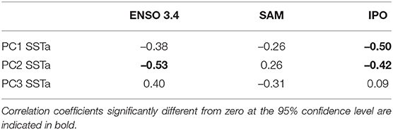
Table 6. Linear correlation coefficients (r) between the PC time series of SSTa in the region spanning 110°-10°W, 60°-10°S and climate indices (ENSO 3.4, SAM, and IPO), for the period 1982–2017 (see Section 4.3).
Moderate but significant correlations are found between PC1 and the IPO (r = –0.50), and between PC2 and the IPO and ENSO 3.4 (r = –0.42 and –0.53, respectively). The correlations with SAM are low and non-significant for all PCs. Thus, only moderate correlations are observed between PCs and individual climate indices (Table 6). This suggests that the contribution of these indices to the SSTa variability on the PS is not direct. Because the interest of this work is to explain the interannual variations of SSTa on the PS through its PC, we analyzed the sum of PC1 and PC2 series (PC1+2) which explain 51% of the total variance of the SSTa at SPS and adequately represents the negative and positive SSTa periods. A multiple linear regression was performed to estimate PC1+2 values through the three climatic indices considered (SAM, ENSO 3.4, IPO). This regression significantly correlates (r = 0.63) with PC1+2 and explains 40% of its variance. The coefficients obtained by the multilinear regression are positive for the ENSO 3.4 and IPO indices and negative for SAM. This indicates that during positive ENSO periods, the poleward and eastward propagation of Rossby waves promotes positive values of PC1+2 and therefore positive SSTa at SPS. On the other hand, the relationship with SAM is inverse: when SAM is positive (intensified westerly winds), the northward advection of cold waters in the Ekman layer from the south to the SPS region and increased wind speeds enhance vertical mixing are promoted. In addition, as meridional wind speed variability around southern South America is negatively correlated with SAM index (r = −0.52) (Guihou et al., 2020), during positive SAM index periods, southerly winds can partially induce cross-shore pressure gradient and an anomalous northward geostrophic transport. These factors will likely promote negative PC1+2 anomalies and negative SSTa at SPS.
This simplified multilinear regression model provides a first approach to assess the teleconnection mechanisms that are relevant for the interannual variations of SSTa on the PS. Furthermore, since the global patterns considered have a certain degree of predictability on interannual time scales (Newman, 2007), it is possible to estimate, at least, the sign of regional SSTa.
4. Discussion
We analyzed linear trends and the interannual variability of SST anomaly fluctuations over the Southeastern Pacific and the Southwestern Atlantic focused on the variability over the productive Atlantic Patagonian continental shelf. The possible link between SSTa variability and local and large-scale atmospheric forcing from 1982 to 2017 was investigated using satellite and reanalysis databases. Intense positive SSTa linear trends are observed along the Brazil Current and the Brazil-Malvinas Confluence (> 0.4°C decade−1), while negative trends (< –0.2°C decade−1) are observed in the northernmost extension of the Malvinas Current. This meridional dipole pattern in the linear trend of SST extends over the continental shelf of the western South Atlantic, where significant positive trends north of 46°S and negative trends south of 49°S are observed. For our analysis we selected two areas of significant warming and cooling trends on the PS (NPS and SPS, respectively). We found that the observed trends in these regions represent variations of almost half a degree, with an increase of 0.52°C at NPS and a decrease of –0.42°C at SPS and that they are mostly associated with the variability observed during the past decade (2008–2017). During 2008–2017, the positive SSTa trend at NPS is strongly correlated with a decrease in the local zonal wind, i.e., to a local decline of the strength of westerly winds (r = –0.85). The SSTa variability at SPS is significantly correlated with the meridional wind (r = –0.61). This is consistent with enhanced southerly winds that reinforce northward geostrophic advection anomalies of cold waters at SPS as suggested by numerical simulations.
We find a strong interannual signal on the PS with periods centered at around 6 years. The first three leading modes of variability (EOF) in the domain bounded by 110–10°W, 10–60°S explain 28, 16, and 12% of the variance, respectively. Our analyses indicate that EOF1 and EOF2 over the above-mentioned domain represent variability associated with SSTa in the southeast Pacific and southwest Atlantic basins, respectively, while EOF3 combines variance from both basins. The sum of PC1 and PC2 (PC1+2) is significantly correlated with detrended SSTa (r = 0.71) and explains 51% of the variance at SPS. A multiple linear regression was performed including SAM, ENSO 3.4, IPO indices. This regression is significantly correlated (r = 0.63) with PC1+2 suggesting that during positive ENSO periods, the poleward propagation of atmospheric Rossby waves modulates the zonal and meridional wind variability generating anticyclonic wind anomalies (u-wnda <0 and v-wnda > 0) that promote positive values of PC1+2 and therefore positive SSTa at SPS. In addition, the relationship with SAM is inverse: when SAM is positive (intensified westerly winds), the northward advection of cold waters to the SPS region is promoted and is further increased by intensified wind speeds that enhance vertical mixing. These two factors promote negative PC1+2 anomalies, that is negative SSTa in the SPS region. These results suggest that the SST variability observed around southern South America is partially modulated by the PDO, ENSO 3.4 and SAM, which indicate a linkage with the variability of the east-central Pacific.
To summarize, we have developed a comprehensive analysis whereby the SSTa interannual variability and trends on the SEP and SWA are forced by a combination of local and remote processes, with trends on the PS explained by local winds during the past 10 years of the records and interannual variability caused by a combination of IPO, ENSO and SAM.
Data Availability Statement
The original contributions presented in the study are included in the article/Supplementary Material, further inquiries can be directed to the corresponding author.
Author Contributions
DR, MPC, and AP contributed substantially to the design of this study, the analysis of the data, drafting the work, interpreting results and revising it critically. All authors have approved the final version and agreed to be accountable for all aspects of the work in ensuring that questions related to the accuracy or integrity of any part of the work are appropriately investigated and resolved.
Funding
This work was carried out with the aid of a grant from the Inter-American Institute for Global Change Research (IAI) CRN3070 which is supported by the U.S. National Science Foundation (grant no. GEO-1128040) and IAI grant no. SGP-HW 017.
Conflict of Interest
The authors declare that the research was conducted in the absence of any commercial or financial relationships that could be construed as a potential conflict of interest.
Publisher's Note
All claims expressed in this article are solely those of the authors and do not necessarily represent those of their affiliated organizations, or those of the publisher, the editors and the reviewers. Any product that may be evaluated in this article, or claim that may be made by its manufacturer, is not guaranteed or endorsed by the publisher.
Supplementary Material
The Supplementary Material for this article can be found online at: https://www.frontiersin.org/articles/10.3389/fmars.2022.829144/full#supplementary-material
References
Abram, N., Gattuso, J.-P., Prakash, A., Cheng, L., Chidichimo, M. P., Crate, S., et al. (2019). “Framing and context of the report,” in IPCC Special Report on the Ocean and Cryosphere in a Changing Climate, Chapter 1, 73–129. Available online at: https://www.ipcc.ch/srocc/chapter/chapter-1-framing-and-context-of-the-report/
Acha, E. M., Mianzan, H. W., Guerrero, R. A., Favero, M., and Bava, J. (2004). Marine fronts at the continental shelves of austral South America: physical and ecological processes. J. Mar. Syst. 44, 83–105. doi: 10.1016/j.jmarsys.2003.09.005
Atlas, R., Hoffman, R. N., Ardizzone, J., Leidner, S. M., Jusem, J. C., Smith, D. K., et al. (2011). A cross-calibrated, multiplatform ocean surface wind velocity product for meteorological and oceanographic applications. Bull. Am. Meteorol. Soc. 92, 157–174. doi: 10.1175/2010BAMS2946.1
Bao, X., and Zhang, F. (2013). Evaluation of NCEP-CFSR, NCEP-NCAR, ERA-Interim, and ERA-40 reanalysis datasets against independent sounding observations over the Tibetan Plateau. J. Clim. 26, 206–214. doi: 10.1175/JCLI-D-12-00056.1
Beaugrand, G., and Reid, P. C. (2003). Long-term changes in phytoplankton, zooplankton and salmon related to climate. Glob. Chang Biol. 9, 801–817. doi: 10.1046/j.1365-2486.2003.00632.x
Bindoff, N. L., Cheung, W. W., Kairo, J. G., Arístegui, J., Guinder, V. A., Hallberg, R., et al. (2019). “Changing ocean, marine ecosystems, and dependent communities,” in IPCC Special Report on the Ocean and Cryosphere in a Changing Climate, Chapter 5, 477–587. Available online at: https://www.ipcc.ch/srocc/chapter/chapter-5/
Bisbal, G. A. (1995). The Southeast South American shelf large marine ecosystem: evolution and components. Mar. Policy 19, 21–38. doi: 10.1016/0308-597X(95)92570-W
Cheng, L., Abraham, J., Zhu, J., Trenberth, K. E., Fasullo, J., Boyer, T., et al. (2020). Record-setting ocean warmth continued in 2019. Adv. Atmosphere. Sci. 37, 137–142. doi: 10.1007/s00376-020-9283-7
Church, J. A., Clark, P. U., Cazenave, A., Gregory, J. M., Jevrejeva, S., Levermann, A., et al. (2013). Sea level change. Technical report, PM Cambridge University Press.
Ciais, P., Sabine, C., Bala, G., Bopp, L., Brovkin, V., Canadell, J., et al. (2014). “Carbon and other biogeochemical cycles,” in Climate change 2013: the physical science basis. Contribution of Working Group I to the Fifth Assessment Report of the Intergovernmental Panel on Climate Change, Chapter 6 (Cambridge; New York, NY: Cambridge University Press), 465–570.
Combes, V., and Matano, R. P. (2018). The Patagonian shelf circulation: drivers and variability. Prog Oceanogr. 167, 24–43. doi: 10.1016/j.pocean.2018.07.003
Dee, D. P., Uppala, S. M., Simmons, A., Berrisford, P., Poli, P., Kobayashi, S., et al. (2011). The ERA-Interim reanalysis: configuration and performance of the data assimilation system. Q. J. R. Meteorol. Soc. 137, 553–597. doi: 10.1002/qj.828
Deser, C., Alexander, M. A., Xie, S.-P., and Phillips, A. S. (2010). Sea surface temperature variability: patterns and mechanisms. Ann. Rev. Mar. Sci. 2, 115–143. doi: 10.1146/annurev-marine-120408-151453
Doney, S. C., Ruckelshaus, M., Emmett Duffy, J., Barry, J. P., Chan, F., English, C. A., et al. (2012). Climate change impacts on marine ecosystems. Ann. Rev. Mar. Sci. 4, 11–37. doi: 10.1146/annurev-marine-041911-111611
Dong, B., Sutton, R. T., and Scaife, A. A. (2006). Multidecadal modulation of El Ni no-Southern Oscillation (ENSO) variance by Atlantic Ocean sea surface temperatures. Geophys. Res. Lett. 33, 1–4. doi: 10.1029/2006GL025766
Falabella, V., Campagna, C., and Croxall, J. (2009). Atlas del mar patagónico. Especies y espacios. Wildlife Conservation Society, Argentina, and BirdLife International: Buenos Aires.). Available online at: http://www.atlas-marpatagonico.org.
Fan, T., Deser, C., and Schneider, D. P. (2014). Recent Antarctic sea ice trends in the context of Southern Ocean surface climate variations since 1950. Geophys. Res. Lett. 41, 2419–2426. doi: 10.1002/2014GL059239
Garcí-Serrano, J., Cassou, C., Douville, H., Giannini, A., and Doblas-Reyes, F. J. (2017). Revisiting the ENSO teleconnection to the tropical North Atlantic. J. Clim. 30, 6945–6957. doi: 10.1175/JCLI-D-16-0641.1
Garreaud, R. D., Clem, K., and Veloso, J. V. (2021). The South Pacific pressure trend dipole and the southern blob. J. Clim. 34, 7661–7676. doi: 10.1175/JCLI-D-20-0886.1
Gianelli, I., Ortega, L., Marín, Y., Piola, A. R., and Defeo, O. (2019). Evidence of ocean warming in Uruguay's fisheries landings: the mean temperature of the catch approach. Mar. Ecol. Prog. Ser. 625, 115–125. doi: 10.3354/meps13035
Glorioso, P. D., and Flather, R. A. (1995). A barotropic model of the currents off SE South America. J. Geophys. Res. Oceans 100, 13427–13440. doi: 10.1029/95JC00942
Gordon, A. L., and Greengrove, C. L. (1986). Geostrophic circulation of the Brazil-Falkland confluence. Deep Sea Res. A Oceanogr. Res. Pap. 33, 573–585. doi: 10.1016/0198-0149(86)90054-3
Goyal, R., England, M. H., Jucker, M., and Gupta, A. S. (2021). Response of Southern Hemisphere western boundary current regions to future zonally symmetric and asymmetric atmospheric changes. J. Geophys. Res. Oceans 126, e2021JC017858. doi: 10.1029/2021JC017858
Guihou, K., Piola, A. R., Palma, E. D., and Chidichimo, M. P. (2020). Dynamical connections between large marine ecosystems of austral South America based on numerical simulations. Ocean Sci. 16, 271–290. doi: 10.5194/os-16-271-2020
Hall, A., and Visbeck, M. (2002). Synchronous variability in the Southern Hemisphere atmosphere, sea ice, and ocean resulting from the annular mode. J. Clim. 15, 3043–3057. doi: 10.1175/1520-0442(2002)015<3043:SVITSH>2.0.CO;2
Hardiman, S., Dunstone, N., Scaife, A., Smith, D., Ineson, S., Lim, J., et al. (2019). The impact of strong El Ni no and La Ni na events on the North Atlantic. Geophys. Res. Lett. 46, 2874–2883. doi: 10.1029/2018GL081776
Hartmann, D. L., Tank, A. M. K., Rusticucci, M., Alexander, L. V., Brönnimann, S., Charabi, Y. A. R., et al. (2013). “Observations: atmosphere and surface,” in Climate Change 2013 the Physical Science Basis: Working Group I Contribution to the Fifth Assessment Report of the Intergovernmental Panel on Climate Change, Chapter 2 (Cambridge; New York, NY: Cambridge University Press), 159–254.
Hays, G. C., Richardson, A. J., and Robinson, C. (2005). Climate change and marine plankton. Trends Ecol. Evolut. 20, 337–344. doi: 10.1016/j.tree.2005.03.004
Henley, B. J., Gergis, J., Karoly, D. J., Power, S., Kennedy, J., and Folland, C. K. (2015). A tripole index for the Interdecadal Pacific oscillation. Clim. Dyn. 45, 3077–3090. doi: 10.1007/s00382-015-2525-1
Hirsch, R. M., Alexander, R. B., and Smith, R. A. (1991). Selection of methods for the detection and estimation of trends in water quality. Water Resour. Res. 27, 803–813. doi: 10.1029/91WR00259
Hobday, A. J., Alexander, L. V., Perkins, S. E., Smale, D. A., Straub, S. C., Oliver, E. C., et al. (2016). A hierarchical approach to defining marine heatwaves. Prog. Oceanogr. 141, 227–238. doi: 10.1016/j.pocean.2015.12.014
Hobday, A. J., and Pecl, G. T. (2014). Identification of global marine hotspots: sentinels for change and vanguards for adaptation action. Rev. Fish. Biol. Fish. 24, 415–425. doi: 10.1007/s11160-013-9326-6
Ishii, M., Fukuda, Y., Hirahara, S., Yasui, S., Suzuki, T., and Sato, K. (2017). Accuracy of global upper ocean heat content estimation expected from present observational data sets. Sola 13, 163–167. doi: 10.2151/sola.2017-030
Johnson, G. C., and Lyman, J. M. (2020). Warming trends increasingly dominate global ocean. Nat. Clim. Chang 10, 757–761. doi: 10.1038/s41558-020-0822-0
Kalnay, E., Kanamitsu, M., Kistler, R., Collins, W., Deaven, D., Gandin, L., et al. (1996). The NCEP/NCAR 40-year reanalysis project. Bull. Am. Meteorol. Soc. 77, 437–472. doi: 10.1175/1520-0477(1996)077<0437:TNYRP>2.0.CO;2
Kayano, M. T., and Capistrano, V. B. (2014). How the Atlantic multidecadal oscillation (AMO) modifies the ENSO influence on the South American rainfall. Int. J. Climatol. 34, 162–178. doi: 10.1002/joc.3674
Kim, Y. S., and Orsi, A. H. (2014). On the variability of Antarctic circumpolar current fronts inferred from 1992-2011 altimetry. J. Phys. Oceanogr. 44, 3054–3071. doi: 10.1175/JPO-D-13-0217.1
Kostov, Y., Ferreira, D., Armour, K. C., and Marshall, J. (2018). Contributions of greenhouse gas forcing and the southern annular mode to historical southern ocean surface temperature trends. Geophys. Res. Lett. 45, 1086–1097. doi: 10.1002/2017GL074964
Lago, L., Saraceno, M., Martos, P., Guerrero, R., Piola, A., Paniagua, G., et al. (2019). On the wind contribution to the variability of ocean currents over wide continental shelves: a case study on the northern argentine continental shelf. J. Geophys. Res. Oceans 124, 7457–7472. doi: 10.1029/2019JC015105
Le Quéré, C., Andrew, R. M., Friedlingstein, P., Sitch, S., Hauck, J., Pongratz, J., et al. (2018). Global carbon budget 2018. Earth Syst. Sci. Data 10, 2141–2194. doi: 10.5194/essd-10-2141-2018
Lee, S.-K., Enfield, D. B., and Wang, C. (2008). Why do some El Ni nos have no impact on tropical North Atlantic SST? Geophys. Res. Lett. 35(16). doi: 10.1029/2008GL034734
Liléo, S., Berge, E., Undheim, O., Klinkert, R., and Bredesen, R. E. (2013). Long-term correction of wind measurements. State-of-the-art, guidelines and future work. Elforsk Rep. 13, 18. Available online at: https://energiforskmedia.blob.core.windows.net/media/19814/long-term-correction-of-wind-measurements-elforskrapport-2013-18.pdf
Ling, S., Johnson, C., Ridgway, K., Hobday, A., and Haddon, M. (2009). Climate-driven range extension of a sea urchin: inferring future trends by analysis of recent population dynamics. Glob. Chang Biol. 15, 719–731. doi: 10.1111/j.1365-2486.2008.01734.x
Lledó, L., Lead, T., and Dubois, J. (2013). A study of wind speed variability using global reanalysis data. AWS Truepower technical report, 137–142.
Mann, H. B. (1945). Nonparametric tests against trend. Econometrica 13, 245–259. doi: 10.2307/1907187
Matano, R., Palma, E. D., and Piola, A. R. (2010). The influence of the Brazil and malvinas currents on the southwestern atlantic shelf circulation. Ocean Sci. 6, 983–995. doi: 10.5194/os-6-983-2010
McLeod, A. I., Hipel, K. W., and Bodo, B. A. (1991). Trend analysis methodology for water quality time series. Environmetrics 2, 169–200. doi: 10.1002/env.3770020205
Meredith, M. P., Murphy, E. J., Hawker, E. J., King, J. C., and Wallace, M. I. (2008). On the interannual variability of ocean temperatures around South Georgia, Southern Ocean: Forcing by El Ni no-Southern Oscillation and the Southern Annular Mode. Deep Sea Res. II Top. Stud. Oceanogr. 55, 2007–2022. doi: 10.1016/j.dsr2.2008.05.020
Messié, M., and Chavez, F. (2011). Global modes of sea surface temperature variability in relation to regional climate indices. J. Clim. 24, 4314–4331. doi: 10.1175/2011JCLI3941.1
Mezzina, B., García-Serrano, J., Bladé, I., and Kucharski, F. (2020). Dynamics of the ENSO teleconnection and NAO variability in the north atlantic-european late winter. J. Clim. 33, 907–923. doi: 10.1175/JCLI-D-19-0192.1
Muller-Karger, F. E., Kavanaugh, M. T., Montes, E., Balch, W. M., Breitbart, M., Chavez, F. P., et al. (2014). A framework for a marine biodiversity observing network within changing continental shelf seascapes. Oceanography 27, 18–23. doi: 10.5670/oceanog.2014.56
Nerem, R. S., Beckley, B. D., Fasullo, J. T., Hamlington, B. D., Masters, D., and Mitchum, G. T. (2018). Climate-change-driven accelerated sea-level rise detected in the altimeter era. Proc. Natl. Acad. Sci. U.S.A. 115, 2022–2025. doi: 10.1073/pnas.1717312115
Newman, M. (2007). Interannual to Decadal predictability of tropical and North Pacific sea surface temperatures. J. Clim. 20, 2333–2356. doi: 10.1175/JCLI4165.1
Newman, M., Alexander, M. A., Ault, T. R., Cobb, K. M., Deser, C., Di Lorenzo, E., et al. (2016). The pacific decadal oscillation, revisited. J. Clim. 29, 4399–4427. doi: 10.1175/JCLI-D-15-0508.1
Oppenheimer, M., Glavovic, B., Hinkel, J., van de Wal, R., Magnan, A. K., Abd-Elgawad, A., et al. (2019). “Sea level rise and implications for low lying islands, coasts and communities,” in IPCC Special Report on the Ocean and Cryosphere in a Changing Climate, Chapter 4. Available online at: https://www.ipcc.ch/srocc/chapter/chapter-4-sea-level-rise-and-implications-for-low-lying-islands-coasts-and-communities/
Oschlies, A., Brandt, P., Stramma, L., and Schmidtko, S. (2018). Drivers and mechanisms of ocean deoxygenation. Nat. Geosci. 11, 467–473. doi: 10.1038/s41561-018-0152-2
Palma, E. D., Matano, R. P., and Piola, A. R. (2008). A numerical study of the Southwestern Atlantic Shelf circulation: Stratified ocean response to local and offshore forcing. J. Geophys. Res. Oceans 113, C11010. doi: 10.1029/2007JC004720
Palma, E. D., Matano, R. P., Piola, A. R., and Sitz, L. E. (2004). A comparison of the circulation patterns over the Southwestern Atlantic Shelf driven by different wind stress climatologies. Geophys. Res. Lett. 31, 1–5. doi: 10.1029/2004GL021068
Parmesan, C., and Yohe, G. (2003). A globally coherent fingerprint of climate change impacts across natural systems. Nature 421, 37–42. doi: 10.1038/nature01286
Pecl, G. T., Ward, T. M., Doubleday, Z. A., Clarke, S., Day, J., Dixon, C., et al. (2014). Rapid assessment of fisheries species sensitivity to Climate Change. Clim. Change 127, 505–520. doi: 10.1007/s10584-014-1284-z
Piola, A. R., Palma, E. D., Bianchi, A. A., Castro, B. M., Dottori, M., Guerrero, R. A., et al. (2018). “Physical oceanography of the SW Atlantic Shelf: a review,” in Plankton Ecology of the Southwestern Atlantic (Cham: Springer), 37–56.
Preisendorfer, R. W., and Mobley, C. D. (1988). Principal component analysis in meteorology and oceanography. Dev. Atmosphere. Sci. 17, 425.
Ramírez, F., Afán, I., Davis, L. S., and Chiaradia, A. (2017). Climate impacts on global hot spots of marine biodiversity. Sci. Adv. 3, e1601198. doi: 10.1126/sciadv.1601198
Reynolds, R. W., Smith, T. M., Liu, C., Chelton, D. B., Casey, K. S., and Schlax, M. G. (2007). Daily high-resolution-blended analyses for sea surface temperature. J. Clim. 20, 5473–5496. doi: 10.1175/2007JCLI1824.1
Rhein, M., Rintoul, S. R., Aoki, S., Campos, E., Chambers, D., Feely, R. A., et al. (2013). “Observations: ocean,” in Climate Change 2013: The Physical Science Basis. Contribution of Working Group I to the Fifth Assessment Report of the Intergovernmental Panel on Climate Change, eds T. Stocker, D. P. G. -K. Qin, M. Tignor, S. Allen, J. Boschung, A. Nauels, Y. Xia, V. Bex, and P. Midgley (Cambridge: Cambridge University Press), 255–316.
Rivadeneira, M. M., and Fernández, M. (2005). Shifts in southern endpoints of distribution in rocky intertidal species along the south-eastern Pacific coast. J. Biogeogr. 32, 203–209. doi: 10.1111/j.1365-2699.2004.01133.x
Rivas, A. L. (1994). Spatial variation of the annual cycle of temperature in the Patagonian shelf between 40 and 50 of south latitude. Cont. Shelf Res. 14, 1539–1554. doi: 10.1016/0278-4343(94)90089-2
Rivas, A. L. (2010). Spatial and temporal variability of satellite-derived sea surface temperature in the southwestern Atlantic Ocean. Cont. Shelf Res. 30, 752–760. doi: 10.1016/j.csr.2010.01.009
Rodrigues, R. R., Campos, E. J., and Haarsma, R. (2015). The impact of ENSO on the South Atlantic subtropical dipole mode. J. Clim. 28, 2691–2705. doi: 10.1175/JCLI-D-14-00483.1
Romero, S. I., Piola, A. R., Charo, M., and Garcia, C. A. E. (2006). Chlorophyll-a variability off Patagonia based on SeaWiFS data. J. Geophys. Res. Oceans 111, 1–11. doi: 10.1029/2005JC003244
Saha, S., Moorthi, S., Pan, H.-L., Wu, X., Wang, J., Nadiga, S., et al. (2010). The NCEP climate forecast system reanalysis. Bull. Am. Meteorol. Soc. 91, 1015–1058. doi: 10.1175/2010BAMS3001.1
Stramma, L., Prince, E. D., Schmidtko, S., Luo, J., Hoolihan, J. P., Visbeck, M., et al. (2012). Expansion of oxygen minimum zones may reduce available habitat for tropical pelagic fishes. Nat. Clim. Chang. 2, 33–37. doi: 10.1038/nclimate1304
Thompson, D. W., and Wallace, J. M. (2000). Annular modes in the extratropical circulation. Part I: Month-to-month variability. J. Clim. 13, 1000–1016. doi: 10.1175/1520-0442(2000)013<1000:AMITEC>2.0.CO;2
Thomson, R. E., and Emery, W. J. (2014). Data Analysis Methods in Physical Oceanography, 3rd Edn. Waltham, MA: Newnes.
Turner, J. (2004). The El Niño Southern Oscillation and Antarctica. Int. J. Climatol. 24, 1–31. doi: 10.1002/joc.965
Von Schuckmann, K., Le Traon, P.-Y., Alvarez-Fanjul, E., Axell, L., Balmaseda, M., Breivik, L.-A., et al. (2016). The copernicus marine environment monitoring service ocean state report. J. Operat. Oceanogr. 9(Suppl. 2):S235–S320. doi: 10.1080/1755876X.2016.1273446
Von Schuckmann, K., Le Traon, P.-Y., Smith, N., Pascual, A., Brasseur, P., Fennel, K., et al. (2018). Copernicus marine service ocean state report. J. Operat. Oceanogr. 11(Suppl. 1):S1–S142.
Walther, G.-R., Post, E., Convey, P., Menzel, A., Parmesan, C., Beebee, T. J., et al. (2002). Ecological responses to recent climate change. Nature 416, 389–395. doi: 10.1038/416389a
Welch, P. (1967). The use of fast Fourier transform for the estimation of power spectra: a method based on time averaging over short, modified periodograms. IEEE Trans. Audio Electroacoust. 15, 70–73. doi: 10.1109/TAU.1967.1161901
Wentz, F., Scott, J., Hoffman, R., Leidner, M., Atlas, R., and Ardizzone, J. (2015). Remote Sensing Systems Cross-Calibrated Multi-Platform (CCMP) 6-hourly ocean vector wind analysis product on 0.25 deg grid, Version 2.0. Santa Rosa, CA: Remote Sensing Systems.
Yang, H., Lohmann, G., Krebs-Kanzow, U., Ionita, M., Shi, X., Sidorenko, D., et al. (2020). Poleward shift of the major ocean gyres detected in a warming climate. Geophys. Res. Lett. 47, e2019GL085868. doi: 10.1029/2019GL085868
Keywords: sea surface temperature, Southwest South Atlantic, interannual variability, climate variability, trends, sea-air interaction, atmospheric forcing
Citation: Risaro DB, Chidichimo MP and Piola AR (2022) Interannual Variability and Trends of Sea Surface Temperature Around Southern South America. Front. Mar. Sci. 9:829144. doi: 10.3389/fmars.2022.829144
Received: 05 December 2021; Accepted: 02 February 2022;
Published: 04 March 2022.
Edited by:
Regina R. Rodrigues, Federal University of Santa Catarina, BrazilReviewed by:
Wlademir Santis, University of São Paulo, BrazilPaola M. Castellanos, European University of Lisbon, Portugal
Copyright © 2022 Risaro, Chidichimo and Piola. This is an open-access article distributed under the terms of the Creative Commons Attribution License (CC BY). The use, distribution or reproduction in other forums is permitted, provided the original author(s) and the copyright owner(s) are credited and that the original publication in this journal is cited, in accordance with accepted academic practice. No use, distribution or reproduction is permitted which does not comply with these terms.
*Correspondence: Daniela B. Risaro, drisaro@at.fcen.uba.ar