Combining Models of Environment, Behavior, and Physiology to Predict Tissue Hydrogen and Oxygen Isotope Variance Among Individual Terrestrial Animals

Introduction

Variations in stable hydrogen (δ²H) and oxygen (δ¹⁸O) isotopic ratios of animal body tissues are commonly used in terrestrial migration ecology to reconstruct origin and migration (reviewed by Hobson, 1999; Hobson and Wassenaar, 2019). The underlying premise of this method is that the isotopic compositions of body tissues are linked to those of local precipitation through predictable relationships (e.g., Chamberlain et al., 1996; Hobson and Wassenaar, 1997; Hobson et al., 2004; but see Hobson et al., 2012; Nordell et al., 2016; Magozzi et al., 2019). Because the isotopic composition of precipitation varies predictably across space and time (Craig, 1961; Bowen and Revenaugh, 2003; for a review see Bowen, 2010), variations in tissue isotopic compositions can be compared with spatial patterns in precipitation isotope ratios (isoscapes; e.g., Bowen et al., 2005b) to infer differences in tissue origin or migration. For example, bird feather δ²H values have been widely used to constrain the location of molting grounds (Chamberlain et al., 1996; Hobson and Wassenaar, 1997; Kelly et al., 2002; Hobson et al., 2004; Rubenstein and Hobson, 2004; reviewed by Hobson and Wassenaar, 2019). Oxygen isotope ratios are often measured simultaneously with δ²H values, and can also potentially provide useful information on molt location (Hobson et al., 2004, 2019; Hobson and Koehler, 2015).

A key premise underpinning the utilization of isotope-based methods to infer origin and migration is that tissue grown at the same site are isotopically similar. However, isotopic data from known-origin samples commonly show high levels of variation even among conspecific individuals living at a common site (e.g., Kelly et al., 2002; Meehan et al., 2003; Smith and Dufty, 2005; Wunder et al., 2005; Rocque et al., 2006; Langin et al., 2007; Gow et al., 2012; Haché et al., 2012; van Dijk et al., 2014; Reese et al., 2018). Such variability can often be quantified and incorporated in geographic assignment tests (Hobson et al., 2012, 2014) but may limit the utility of such tests. Specifically, where the local isotopic variation is small relative to variation among locations, accurate assignments can be made; as the local variability increases, distributions for geographically distinct populations increasingly overlap and assignments become less certain (Wunder et al., 2005; Wunder, 2010; Hobson et al., 2012). Feather δ²H values of mountain plover (Charadrius montanus) chicks from 20 single breeding sites from Colorado to Montana, for example, spanned an average range of 41‰ across sites (average SD = 12‰; 5 ≤ n ≤ 164; minimum range = 16.3‰; maximum range = 109.2‰; Wunder et al., 2005; Wunder personal communication), severely limiting the use of isotopes to study migration in this species (Wunder et al., 2005). Values of feathers from adult American golden plovers (Pluvialis dominica) presumably grown over a small geographic area in Alaska varied over an even larger range (113‰; mean ± SD = −129 ± 69‰, n = 5; Rocque et al., 2006; but see Larson and Hobson, 2009). For adult American redstarts (Setophaga ruticilla) breeding in southeast Ontario, Canada, in contrast, the local range in feather δ²H values was only as high as 22‰ in 2004 (mean ± SD = −82 ± 4‰, n = 42; Langin et al., 2007) but even in this case assignment tests including local among-individual isotopic variation had reduced resolution (Langin et al., 2007). Over continental scales, within-site taxon-specific δ²H values spanned an average range of 25‰ across 13 sites and eight taxa (average SD = 8‰; 5 ≤ n ≤ 17; minimum range = 4‰ for Hylocichla mustelina; maximum range = 45.1‰ for Catharus ustulatus; Hobson et al., 2012).

Although we have a solid understanding of the processes controlling broad-scale isotope patterns (reviewed by Bowen, 2010), a more fundamental understanding of the underlying mechanisms of small-scale isotope variance is needed to improve estimates of such variance and assess the potential utility of isotope-based methods for specific groups or environments. Several studies have investigated the causes of within-site among-individual isotopic variance through exploratory approaches such as correlation analysis and model selection (e.g., Clegg et al., 2003; Meehan et al., 2003; Smith and Dufty, 2005; Langin et al., 2007; Reese et al., 2018; see also Hobson et al., 2012; Nordell et al., 2016). Relationships between feather δ²H values and age have been observed for several taxa (e.g., Meehan et al., 2003; Smith and Dufty, 2005; Langin et al., 2007; Haché et al., 2012; Studds et al., 2012; Gomez et al., 2019) and attributed to age-related differences in diet, access to water, metabolism (Meehan et al., 2003; Langin et al., 2007; Storm-Suke et al., 2012), and/or evaporative water loss (Wolf and Martinez del Rio, 2000; Meehan et al., 2003, McKechnie et al., 2004; Smith and Dufty, 2005; but see Kirkley and Gessaman, 1990; Marder et al., 2003). Differences in the magnitude and patterns of local among-individual variance observed for shore birds (Wunder et al., 2005; Rocque et al., 2006), raptors (Meehan et al., 2003; Smith and Dufty, 2005), and passerines (Langin et al., 2007) have been attributed to differences in molt phenology and evaporative water loss among these taxa (Smith and Dufty, 2005). Temporal variation in precipitation δ²H has been suggested as a driver of isotopic variation in accipiters (Meehan et al., 2003; Smith and Dufty, 2005). In general, these field-data point to two potential sources of variability: (1) differences in the isotopic composition of the diets of individuals, and (2) differences in individual physiology affecting the transfer of isotopes from diet to tissue. A critical comparison and evaluation of these two mechanisms in the context of empirical and theoretical constraints is lacking.

Discriminating among sources of variance potentially contributing to field-observed data is challenging, especially with incomplete sampling of the spatial and temporal variance in environmental isotope sources, and limited knowledge of the behavior and metabolic status of individuals. Simulation modeling offers an alternative approach, complementary to measurement of tagged individuals or manipulative field-experiments, to explore the potential contributions and interactions of isotope variance-inducing mechanisms to the variance in a sample population. The value of using such an approach is that it allows testing of multiple processes that could contribute to isotopic variation and their interactions, and offers the possibility of conducting experiments in the model environment where each model parameter can be controlled. Simulation models, however, involve assumptions and parameterization, and parameter values may be poorly constrained if data on the movement, behavior, and physiology of the study species are scarce or unavailable. In such cases, simulation using “idealized” models can still provide valuable information on expectations associated with different variance-producing mechanisms or traits, and can be thought of as a framework for generating predictions associated with different hypothesized mechanisms rather than a tool to reproduce actual behavior or physiology. Simulation models of this type have previously been applied to explore how different migration hypotheses may contribute to variation in carbon isotopes in seabirds (Carpenter-Kling et al., 2019) and whales (Trueman and St John Glew, 2019; Trueman et al., 2019) and oxygen isotopes in fish otoliths (Sakamoto et al., 2019).

Here we present a process-based modeling framework to estimate isotopic variation among local, conspecific individuals. The framework combines an agent-based model of animal behavior and movement, a dynamic version of the physiology-biogeochemistry model of Magozzi et al. (2019), and isoscape models of environmental isotopic variability. We use the resulting model toolbox to predict isotopic compositions of individual birds residing at a common but environmentally heterogeneous site, and explore how variation in behavioral, physiological, and environmental traits may interact to produce within-site among-individual isotopic variance. We compare model predictions against data from locally breeding, hatch-year Spotted Towhees (Pipilo maculatus) sampled prior to the start of fall migration in Red Butte Canyon (RBC), Utah, to evaluate which sets of model mechanisms appear most important in producing observed local among-individual isotopic variation.

Materials and Methods

Agent-Based Model

An agent-based (AB) model was developed to simulate the interaction of individual birds with the environment within RBC (Figure 1). The AB model is idealized and does not attempt to fully reproduce bird behavior (and drivers of behavior) but rather is intended to generate a set of ecologically and environmentally plausible hypotheses in order to experimentally manipulate potential sources of variance and explore the resultant effects on the simulated isotopic data. The environmental domain for the AB model was a representation of the spatial distribution of three major habitat types within the canyon: riparian, meadow, and slope (Figure 1). The domain was obtained through (1) classification of LiDAR data (National Ecological Observatory Network, 2017; http://data.neonscience.org) at 1 m by 1 m resolution into four vegetation cover type classes (Supplementary Figure A1), (2) aggregation of vegetation cover type class data to 10 m by 10 m resolution (Supplementary Figure A2), and (3) classification of these data into three habitat type classes (riparian, meadow, and slope; Appendix A). The riparian class comprised closed-canopy valley-bottom forest in the southwest portion of the canyon, including the area around the mist net sites (Figure 1). The meadow habitat represented open-canopy forest with an understory of grasses. Slope habitat included exposed soil, bunch grass, and shrub oak. Grid cell values of other environmental variables that can determine habitat quality (water and tree presence and prey density) were randomly drawn from distributions parameterized depending on habitat type. Water and tree presence were drawn from binomial distributions with probabilities of 50%, 1%, and 0.5% for water presence, and of 40%, 20%, and 5% for tree presence in riparian, meadow, and slope, respectively. Prey density values were obtained by drawing from a gamma distribution with shape and scale parameters giving mean prey densities of 250, 200, and 25 prey items per cell in riparian, meadow, and slope, respectively, and standard deviations of 1/10 of the mean in the former two habitats and of 1/2 of the mean in the latter habitat. Prey density was assumed to be higher in grid cells with trees than in cells without trees, and values drawn for cells with trees were multiplied by a random value drawn from a uniform distribution with min = 1 and max = 10.

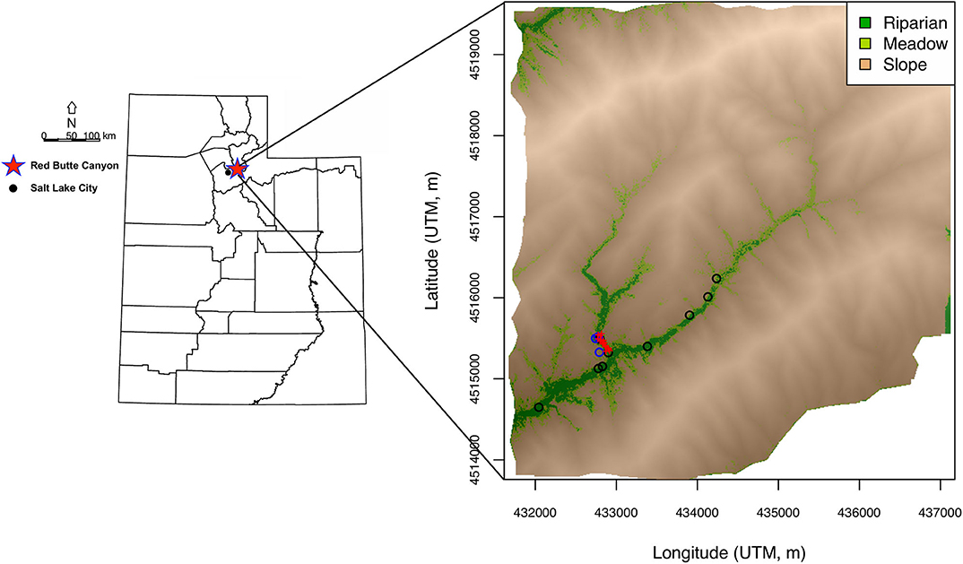
Figure 1. Maps of location of Red Butte Canyon (RBC) within Utah (red star) and spatial distribution of three major habitat types in the canyon: riparian, meadow, and slope. Sampling sites for environmental water (black circles) and prey (blue circles), and locations of mist nets (red pluses) are also shown.

The AB model simulated the movement and behavior of 105 individual birds over 60 days at hourly timesteps. Each bird was assigned a nest location to which it returned periodically over the simulation period. Two sets of simulations were run: in the first set, an equal number of birds (n = 35) were assigned random nesting locations within each habitat, allowing for among-habitat comparisons in the data analysis; in the second set, nesting locations were randomly selected without reference to habitat type, leading to a higher number of birds nesting in the more abundant slope habitat than in the meadow and riparian habitats. Because towhees nest predominantly on or near the ground in shrub-land habitat (https://www.audubon.org/field-guide/bird/spotted-towhee), results from the second set of simulations were considered more representative of the local towhee population and were used in comparisons with the measured feather data.

At each model timestep, an individual makes probabilistic decisions about whether and where to move, whether to drink, or whether to eat. Probabilities of moving, drinking, and eating depend on: (1) time of day, (2) hunger and thirst, and (3) environmental conditions. Thirst and hunger are tracked using two indices, which increase with time since the last drinking and feeding events. The rate of thirst increase during the day is twice that during nighttime, and hunger increase rate during the day is five times higher than at night (Table 1). During the day, thirst increase rate is 7% higher than the “base” rate if in the slope habitat and 7% lower if in the riparian habitat (the base rate applies in meadow habitat). In addition, the rate of thirst increase is 7% higher than the habitat-specific rate if the bird moves, 7% lower if it does not move. Because the flux of vapor water out (F_vw; see below) is ~1/3 of the total water loss for most modeled birds, a 7% shift in thirst growth rate depending on habitat and movement is proportional to a ~20% shift in evaporative water loss (see section Physiology Model). Hunger increase rate (metabolic rate in the physiology model, see below) is 20% higher than the base rate if the animal moves and 20% lower if it does not move. Index values >0 indicate that the birds are thirsty and/or hungry.

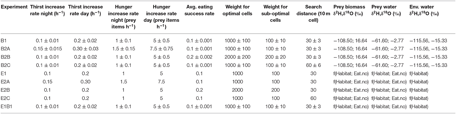
Table 1. Parameter sets for model experiments using combined agent-based and environmental isoscape models.

When present, water is assumed to be available in excess, and therefore every time a bird drinks its thirst index resets to −1. In contrast, food availability is finite, and food intake is determined by food availability in the local environment and the individual's feeding success rate, which are multiplied to obtain a number of prey items eaten per hour; food intake is limited to a maximum of 20 prey items per hour. Eating success rate is randomly drawn from a normal distribution with mean equal to average eating success rate, which is a fixed property for each individual (Table 1), and SD = 0.05; eating success rate has a minimum value of 0.01. When a bird eats, its hunger index decreases in proportion to the number of prey items eaten. As an individual feeds, prey density at the bird's location is concurrently reduced by the number of prey items eaten. Because this work does not focus on competition, the prey density map is re-initialized for each individual.

The probability that a bird will move from its current location depends on whether it is day or night, whether the bird is in its nest, whether it is thirsty and/or hungry, and whether there are adequate local water and/or food resources. At night, a bird that is not in its nest has a 99% probability to move to its nest; a bird that already is in its nest will not move (probability of moving = 0). During the day, a bird that is thirsty and/or hungry but lacks adequate local resources (i.e., water available if thirsty, [how much] food present if hungry) to meet its water and/or food demands has a 90% probability of moving; if resources are adequate, the probability of moving is low (10%). A bird that is neither thirsty nor hungry has a 50% probability to move to its nest (20% chance) or to any cell within the search area (i.e., random exploratory movement; 80% chance). When moving, a bird selects a destination cell within a square search area around its location (Table 1). Within the search area, optimal cells are defined as those that meet the individual's water and/or food requirements (i.e., if a bird is both thirsty and hungry, optimal cells are those with both water and adequate food), suboptimal cells are those that partially meet requirements (i.e., cells with either water or adequate food), and poor cells as those that do not meet any requirement (i.e., cells with neither water nor adequate food). The probability that an individual selects any given cell is proportional to a random variable drawn from distributions shifted to lower values for less desirable cells (Table 1).

The AB model was coupled offline with a physiology-biochemistry model that predicts the H and O isotopic compositions of animal body water and keratins from flux and isotopic inputs to the individual's body (Magozzi et al., 2019). Outputs from the AB model, including time of the day, whether movement and drinking occur, and the number of prey items eaten, were used to define H and O mass fluxes in the physiology model. The individual's location was tracked throughout the AB simulations and used to specify the H and O isotopic compositions of water and food consumed at each timestep based on environmental isoscape models for RBC.

Environmental Isoscape Models

Idealized high-resolution (10 m by 10 m) isoscapes were generated to represent spatial variation in H and O isotopic compositions of environmental water, liquid water within prey items, and prey biomass within RBC. Isoscape models simulated H and O isotope ratios of these resources in each grid cell as a function of habitat and were based on a combination of empirical data and theoretical considerations. Environmental water δ²H and δ¹⁸O grid cell values in the riparian habitat were drawn from a multivariate normal distribution the parameters of which were estimated from H and O isotopic data for 29 streamwater samples from Red Butte Creek downloaded from the Waterisotopes Database (Waterisotopes Database, 2018; http://waterisotopesDB.org) (Figure 1). Standing water is scarce outside the riparian corridor, but the AB model assumes that sparse water resources, for example small puddles or leaf-intercepted water, are available in a subset of grid cells in the meadow and slope habitats. Environmental water δ²H and δ¹⁸O values in these cells were simulated by drawing from the riparian distribution and adding ²H- and ¹⁸O-offsets representing evaporative enrichment. Values of ¹⁸O-enrichment were drawn from a normal distribution with mean = 2‰ for meadow, and mean = 6‰ for slope, and SD = 1/2 of the mean for both habitats. ²H-enrichments were estimated from ¹⁸O-enrichments by assuming an evaporation line with a slope of 4–5 (uniform distribution with min = 4 and max = 5). Thus, both means and variances for environmental water increased from riparian to meadow and slope habitats (Supplementary Figure A7), reflecting the expectation of greater and more variable evaporation of sparse and transient water resources in the latter habitats.

Isoscape models for prey water and prey biomass δ²H and δ¹⁸O values were informed by data for insects and arthropods collected in 1 m by 1 m plots in each habitat at three times during the nesting season (Figure 1). Prey items were collected during the day, which is when the towhees forage, to obtain a relatively representative sample of potential dietary items. Diurnal or seasonal changes in prey activity, however, and the possibility that towhees might forage on some plant material (but see Smith and Greenlaw, 2015; https://birdsna.org/Species-Account/bna/species/spotow), could potentially result in larger isotopic ranges for prey items than those estimated here. Water was cryogenically extracted from individual prey items where possible, or from pooled samples including functionally and taxonomically related species where necessary, and analyzed for H and O isotope ratios using a Picarro L2130-i analyzer. The residual solid mass was homogenized using a mortar and pestle, lipid-extracted in a 2:1 chloroform:methanol solution, allowed to equilibrate with ambient water vapor alongside three keratin standards, vacuum desiccated, and analyzed for isotopic ratios using a Thermo Fisher TC/EA coupled with a Delta V isotope ratio mass spectrometer (for details, see analysis of feather samples). The 1σ precisions for δ²H and δ¹⁸O analyses for water samples were 0.8‰ and 0.25‰, respectively, and for solid mass samples were 2‰ and 0.3‰, respectively. Because sample numbers were relatively small (i.e., prey water: N = 9 in riparian, N = 4 in meadow, and N = 3 in slope), we chose to analyze these data in terms of isotopic offsets between substrates and habitats rather than using the raw data to characterize prey biomass and prey water isotope distributions directly (for plots of raw data, see Appendix A). For prey water, like for environmental water, evaporation is the primary process expected to produce isotopic differentiation among habitats. We estimated the ¹⁸O-enrichment between prey water (δ¹⁸O_pw) and average stream water (δ¹⁸O_streamw) in each habitat, and thus calculated δ¹⁸O_pw values as:

Maximum possible ¹⁸O-enrichment (ε_{evap, max}) was given by the difference between the most ¹⁸O-enriched prey water sample (across habitats) and the average stream water δ¹⁸O value. Percent enrichment (ε_{evap, %}) – and thus prey water δ²H and δ¹⁸O values – in each grid cell were modeled using a beta distribution with α = 2 and β = 4 for riparian (most samples have small evaporative effects, few samples have large effects), α = β = 2 for meadow, and α = 4 and β = 2 for slope. Prey water δ²H values were estimated from δ¹⁸O values by using a regression line fit to the measured prey water H and O isotope data (Supplementary Figure A4) and adding dispersion by drawing from the residual distribution. The resulting distributions of simulated prey water δ²H and δ¹⁸O data reasonably approximated patterns in measured prey water data: prey water δ²H and δ¹⁸O values increased from riparian to meadow to slope, and among-sample isotopic variance was relatively similar across habitats (Supplementary Figures A3, A7).

Data for field-collected prey samples were standardized for variation in H content, likely related to residual lipid content (details in Appendix A, section 2; Supplementary Figure A5). Prey biomass δ²H and δ¹⁸O data were grouped for functionally and taxonomically similar organisms, and averaged for each habitat. For each functional group, H and O isotopic offsets were calculated for each pair of habitats (Appendix A, section 2; Supplementary Table A1). Comparisons within functional groups showed ²H- and ¹⁸O-enrichment from riparian to meadow to slope (Supplementary Table A1; Supplementary Figure A6), consistent with the expectation that differences in evaporative enrichment of prey body water should translate to differences in the isotope ratios of prey body tissues. Because the numbers of pooled samples and sampled groups varied substantially among habitats (i.e., ant: N = 1 in riparian, N = 1 in meadow, N = 1 in slope; Hemiptera: N = 2 in meadow, N = 2 in slope; fly: N = 1 in riparian, N = 2 in meadow, N = 1 in slope; salbug: N = 1 in riparian, N = 1 in meadow, N = 1 in slope; beetle: N = 3 in riparian, N = 2 in meadow, N = 1 in slope; spider: N = 1 in riparian, N = 2 in meadow), data from the meadow habitat (which was the most extensively sampled for prey) were used to characterize a multivariate normal reference distribution. Grid cell prey biomass δ²H and δ¹⁸O values for all habitats were drawn from this distribution, and values for cells in the riparian and slope habitats were then shifted by the mean within-functional group isotopic offsets for those habitats and the meadow. In this work, model isoscapes describing environmental isotopic variability are static with respect to time.

Physiology Model

We adapted the steady state physiology model of Magozzi et al. (2019) to develop a time-explicit model that predicts the H and O isotopic compositions of animal metabolic stores, body water, and keratins. To couple the AB and physiology models, we developed a “resource storage” sub-model representing the transient storage of metabolic resources between ingestion and metabolism. We modeled a single undifferentiated resource pool and did not attempt to track macronutrients separately with the exception that we tracked two O isotopic compositions: that of the carbohydrate + lipid component of the resource pool, and that of its protein component. The isotopic composition of the former is a function only of the isotope ratios of dietary inputs, whereas the latter is affected also by carbonyl-O exchange with water during digestion. The resource storage model is therefore characterized by four equations (Equations 2–5) that describe the change over time in: (1) resource pool size (O₂, mol O₂), (2) ²H content (carbohydrate + fat + protein component; mol ²H₂), (3) oxygen-18 content in the carbohydrate + fat component (mol ¹⁸O₂), and (4) that in the protein component (mol ¹⁸O₂).

O_2in and O_2out (mol O₂ h⁻¹; Equations A1, A11) are fluxes of energy accumulated from eating and energy consumed via metabolism, respectively. The former is proportional to the number of prey eaten, and the latter equals the resting metabolic expenditure times hunger increase rate (therefore depends on time of the day and movement). Given this scaling, the size of O₂ is directly proportional to the individual's hunger index, coupling the AB and physiology models. The resting metabolic expenditure corresponds to the average energy expenditure during one nighttime hour and is estimated from the average energy expenditure during one daytime hour (based on the metabolic theory of ecology and rescaled to approximate measured metabolic rates in songbirds; Tieleman and Williams, 2000) by assuming that daytime metabolic rate is five times higher than nighttime metabolic rate (as for hunger growth rate in the AB model; Appendix A).

RH_p is the H isotopic composition of prey items. RO_pcarb, RO_pfat, and RO_pprot are the O isotope ratios of dietary (prey) carbohydrate, fat, and protein, respectively (Equations A27–A29), and P_carb, P_fat, and P_prot the relative proportions of each macronutrient in the diet (Supplementary Table A2). The O isotopic input for the protein component is calculated from isotope ratios of dietary protein (RO_pprot) and gut water (RO_gw; Equation A38) assuming partial exchange of carbonyl-O with water in the gut during amino acid hydrolysis (Schoeller et al., 1986), where 1 – P_fO is the proportion of O exchanged (Supplementary Table A2). αOc–w is the fractionation factor associated with the interaction between carbonyl-O and water (Supplementary Table A2). Equations 4 and 5 implicitly assume that macronutrients are metabolized in proportion to their abundance in diet, a simplification adopted throughout our modeling. As a result, the proportion of macronutrient O in the resource pool equals that in diet, meaning RO_{res(carb+fat)} = ¹⁸O_{2res(carb+fat)}/(O₂ × (P_carb + P_fat)) and RO_res(prot) = ¹⁸O_2res(prot)/(O₂ × P_prot).

The change over time in (1) body water pool size (H₂O, mol H₂O), (2) ²H content (mol ²H₂), and (3) oxygen-18 content (mol ¹⁸O) is described as:

F_fH and F_fO (mol H₂ h⁻¹ and mol O h⁻¹, respectively; Equations A12, A18) are fluxes in of H and O derived from the breakdown of food molecules by metabolism, F_fw (mol H₂O h⁻¹; Equation A14) is the flux in of liquid water contained within food, F_dw (mol H₂O h⁻¹) that of drinking water, and F_O2 (mol O h⁻¹; Equation A21) that of inhaled oxygen. Food water is acquired discontinuously only when eating occurs; therefore, F_fw depends on the number of prey eaten at the current timestep. Similarly, F_dw depends on whether drinking occurs at the current timestep. F_dw when drinking occurs was set to a fixed value (0.065 mol H₂O h⁻¹) so that the average dynamic F_dw value is similar to that used in the steady state model (Magozzi et al., 2019). F_dw was then rescaled to reflect known body water turnover times in songbirds (Tieleman and Williams, 2000), given the other water fluxes. F_vw (mol H₂O h⁻¹; Equation A16) is the flux out of vapor water, which is calculated from body size and depends on habitat and movement: it is 20% higher than its base value in the slope habitat, 20% lower in the riparian habitat, and 20% higher than the habitat-specific base value if the bird moves, 20% lower if it does not move. F_lw (mol H₂O h⁻¹; Equation 9) is the excretion of liquid water, which is assumed to vary, within bounds, to maintain water balance as follows:

H₂O (mol H₂O) is body water pool size at the current timestep, M (g) is body mass, P_TBW is a minimum threshold for the proportion of body mass that is water, M_wH2O (g mol⁻¹) is the molecular weight of water. The first condition allows for increased liquid water excretion to restore the body water pool to the minimum threshold size with an e-folding time of 0.08 days (i.e., 2 h); the second imposes a minimum F_lw that depletes the body water pool at a rate of 10% of the threshold size per 7 days. F_wasteH and F_wasteO (mol H₂ h⁻¹ and mol O h⁻¹, respectively; Equations A17, A21) are fluxes out of H and O in waste products; F_CO2 (mol O h⁻¹; Equation A22) the flux out of exhaled CO₂. Isotopic inputs for metabolically derived H and O are isotopic ratios of the resource pool including all components (RH_res, RO_res; Equations A30, A33). Inputs for food water correspond to isotopic compositions of prey water (RH_pw, RO_pw; Table 1), and those for drinking water to those of environmental water (RH_ew, RO_ew; Table 1). αH_bw−−vw and αO_bw−−vw are fractionation factors associated with the loss of body water as vapor, αO_atm−−abs that associated with the absorption of atmospheric O by the lungs, and αOCO₂-bw that associated with the loss of body water as exhaled CO₂ (Supplementary Table A2). RH_bw and RO_bw are the isotope ratios of body water at the current model condition, ²H_2bw/H₂O and ¹⁸O_bw/H₂O, respectively. Model parameter values (Supplementary Table A2) were estimated for a generic towhee (for model constants, see Supplementary Table A3).

Differential equations for model state variables were solved using the R package “deSolve” (method used for solving ordinary differential equations: rk4; Soetaert et al., 2010). Variable values were returned at hourly timesteps. The initial resource pool size was set to 15% of body mass, assuming a mass to energy conversion appropriate for an insectivorous diet (Equation A36). Similarly, the initial body water pool size was set to 68% of body weight (Equation 37). Initial values for ²H and oxygen-18 contents in the resource (carbohydrate + fat component and protein component in the case of O) and body water pools were obtained by running a steady state version of the model. Parameters for the “ode” algorithm are outputs from the AB model (i.e., time of the day, number of prey items eaten, whether drinking occurs, and habitat type) at hourly timesteps.

Following Ehleringer et al. (2008), the H isotopic composition of keratin synthesized at each timestep was calculated as:

RH_follw is the H isotopic composition of follicle water, which is a mixture of body water (RH_bw) and metabolic H (RH_res; for P_bw, see Supplementary Table A2). In turn, the H isotope composition of keratin (RH_ker) is a mixture of the resource pool and follicle water. Since no O is considered to be added at the site of keratin formation, the O isotopic composition of newly synthesized keratin (RO_ker) equals that of the protein component of the resource pool (RO_res(prot)) at the time of synthesis.

Model Experiments

Nine model experiments were conducted by running the model system with different parameter sets (Table 1). Behavior, hereafter “B”, experiments included among-individual variation in traits influencing bird behavior and nutritional physiology (thirst and hunger increase rates during the day and at night, average eating success, probability to select optimal and suboptimal cells over poor cells, and search distance) but no environmental isotopic variability. Parameter values were sampled from uniform distributions spanning the mean ± 10%. Although no empirical constraints were available to inform the selected range of values for the behavioral parameters the ±10% range was adequate to assess the nature of any isotope effects associated with this model component; for the physiology parameters, the range adopted here is consistent with reported inter-individual ranges in metabolic rate for many songbirds (Ambrose et al., 1996; Smit and McKechnie, 2015; Cooper et al., 2019). In these experiments the isotopic compositions of water and food resources were the same in all grid cells. Environment, hereafter “E,” experiments included variability in environmental water, prey water, and prey biomass isotopic compositions but no variation in behavioral traits among individuals. At each drinking and feeding event, isotopic inputs were drawn from habitat- and substrate-specific isoscape distributions described above. In the case of feeding, prey water and prey biomass isotopic compositions were means for the number of prey items eaten. For each set of experiments, we ran a reference case in which behavioral parameters were centered on reference values for towhees (B1 and E1), and three tests in which the species-average values of different groups of behavioral parameters were varied to test the sensitivity of the results to differences in the “typical” behavior of individuals. These tests included increased (by 50%) demand for food and water (B2A and E2A), improved (by 100%) foraging success and habitat selection (B2B and E2B), and increased (by 100%) mobility (larger search distance; B2C and E2C). A final experiment, E1B1, included both among-individual behavioral variation and environmental isotopic variability, using the reference values for behavioral parameter means (Table 1).

Feather Collection and Isotopic Analysis

Spotted Towhee was selected as a target species as hatch-year individuals are abundant in RBC over the breeding season. Locally grown feathers from hatch-year towhees were collected in the canyon prior to the start of fall migration in September (Smith and Greenlaw, 2015; https://birdsna.org/Species-Account/bna/species/spotow) in 2013–2016. After hatching in May through July, towhees undergo a first pre-basic molt in April-July, which is complete and occurs in the nest. Between July and October, they undergo a preformative molt on or near breeding grounds, which includes body feathers but (in ca. 60–65% of the individuals) no rectrices or primaries. By sampling the feathers prior to start of fall migration, we eliminated the possibility of collecting feathers from birds that could have hatched somewhere else and used RBC as a stop-over site during migration. Although no home range data exist for hatch-year towhees, it is likely that these birds are tied to their nest location until migration. Birds were captured with mist nets located at the bottom of the canyon, near the river, in riparian, meadow, and slope habitats (for net sites, see Figure 1). For each capture, various meta-data and biological data were recorded, and one or two tail feathers were pulled. Tail feathers are a common choice for analysis in isotopic research, and no evidence exists for significant isotopic differences between tail and flight feathers (e.g., Hobson et al., 2012; Nordell et al., 2016). All handling of wild birds was conducted following state and federal handling protocols and was approved by the University of Utah Institutional Animal Care and Use Committee (number 18-02002).

Feathers from 62 individual birds were processed and analyzed for H and O isotope ratios at the Stable Isotope Ratio Facility for Environmental Research (SIRFER), University of Utah. Feather material was rinsed three times in a 2:1 chloroform:methanol solution to remove lipids. Samples were ground to a fine powder and duplicate 150 μg aliquots were weighed into pre-combusted silver foil capsules for H and O isotope ratio analysis. Because there is partial isotopic exchange of H atoms in protein with atmospheric water vapor, all unknown samples and three reference materials with known δ²H values of non-exchangeable H (Oryx antelope horn from Ethiopia, ORX: δ²H = −48.3‰, δ¹⁸O = 23.45‰; Dall sheep horn from the Alaskan interior, DS: δ²H = −196.1‰, δ¹⁸O = 4.93‰; commercially available powdered keratin, POW: δ²H = −116.0‰, δ¹⁸O = 11.19‰; Chesson, 2012) were allowed to equilibrate with water vapor in the laboratory atmosphere for 7 days, then were vacuum dehydrated prior to isotope analysis (Bowen et al., 2005a). Values used for the reference materials were anchored to the KHS and CBS standards (KHS: δ²H = −54.1‰, δ¹⁸O = 21.21‰; CBS: δ²H = −197.0‰, δ¹⁸O = 2.39‰; Qi et al., 2011; Soto et al., 2017) based on an inter-laboratory round-robin test. Samples and reference materials were transferred to a Zero Blank Autosampler (Costech Analytical) interfaced with a Thermo-chemical Elemental Analyzer (Thermo Fisher Scientific). They were pyrolized at 1400°C in an oxygen-free environment to form H₂ and CO gases, which were chromatographically separated and introduced sequentially into the source of a Delta Plus XL isotope ratio monitoring mass spectrometer (IRMS; Thermo Fisher Scientific). The data for the reference materials were used to calibrate raw measurements of the δ¹⁸O and non-exchangeable δ²H values for unknown samples relative to the VSMOW-SLAP standard scale using the two-point regression-based approach of Wassenaar and Hobson (2003). Analytical precision, based on the repeated analysis of a check reference material (POW), was better than 2‰ and 0.3‰ (1σ) for δ²H and δ¹⁸O values, respectively.

Data Analysis

In order to remove potential influences of initial conditions on state variable values, only outputs over last 30 days of simulation were considered for data analysis. Individual average keratin δ²H and δ¹⁸O values were calculated over this time, the length of which also likely approximates the isotope incorporation time for bird feathers (Hobson, 1999 and refs. there in). Linear regression models were used to examine relationships between keratin isotopic compositions and model variables including body water turnover time, proportion of water influx coming from drinking (vs. food), and mean input flux isotopic ratios. Body water turnover time (h) was calculated as the ratio of individual average body water pool size (H₂O, mol H₂O) to output flux (F_vw + F_wasteH + F_lw; mol H₂O h⁻¹). Mean input flux isotopic composition equals the mean of individual average isotope values for all inputs (e.g., δ_f, δ_fw, δ_dw, and δ¹⁸O_O2 for O), weighted by their relative contributions to the total water flux.

Relationships between keratin isotopic compositions and multiple predictor variables were described by multiple linear regression models of the form Y = β₀ + β₁X₁ + β₂X₂ + β₃X₃ + … + β_iX_i + ε, and visualized with added variable (partial regression) plots, which show the bivariate relationships between the independent variable Y and each of the predictor variables (X_i), conditioned on the other predictors. To compare modeled vs. measured isotopic variances, mean squared deviances of keratin δ²H and δ¹⁸O values were compared among model experiments and data; means, sample variances, SDs, and ranges for individual average keratin δ²H, and δ¹⁸O values were also calculated for each population.

Complete code to run the models and experiments and generate simulated data is available online (Bowen and Magozzi, 2020).

Results

AB Model Results

Nesting location and habitat strongly influenced the habitat(s) in which individuals spend most time (Figure 2). Across experiments and nesting habitats, individuals preferentially occupy the more resource-rich riparian habitat (relative to its spatial coverage). This effect is accentuated in the experiments with higher food and water demands (e.g., B2A), presumably because individuals are more strongly dependent on the high-resource grid cells to meet their requirements. In contrast, slope-nesting birds spend slightly less time in the riparian habitat in the experiments in which foraging success and habitat selectivity and search distance were increased (e.g., B2B and B2C, respectively), reflecting their greater ability to meet their needs without conducting long-range foraging bouts to the riparian zone. Regardless, the dominant pattern in model results is that individuals are strongly tied to their local (nesting) habitat, suggesting that, within the model framework, nest location drives the locations and conditions of foraging for individuals within a local population.

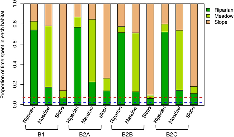
Figure 2. Mean proportion of time spent in each habitat for each experiment (see Table 1) and nesting habitat. Proportions of the study area covered by the riparian habitat (blue dashed line) and by the riparian and meadow habitats (red dashed line) are also shown.

Different habitat utilization could affect the tissue isotopic compositions of individuals in several ways. In the B experiments, among-habitat differences in resource density translate into differing drinking and feeding frequencies and amounts among individuals associated with different habitats. In general, birds associated with the riparian habitat have greater access to water, and therefore drink more frequently than meadow- and slope-nesting birds (Figure 3A), potentially affecting their body water and isotope balance. Riparian nesters also have greater access to adequate food resources to meet their food demands, and therefore eat less frequently but consume greater amounts of food at each feeding event (Figure 3B). In the less resource-rich habitats individuals spend a higher proportion of time actively foraging, particularly in the B2A experiment and slope-nesting individuals in the B2B experiment. Some individuals are unable to obtain sufficient nutrition and completely deplete their resource pool, which we treated here as lethal. Deaths are most common among slope-nesting birds in the B2A and E2A experiments (18 and 16 dead individuals, respectively), due to the increased food demand in these runs. Among-individual variation in drinking and feeding frequencies is, in general, slightly higher for slope-nesting birds than others across the B experiments (Figure 3).

Figure 3. Boxplots of drinking (A) and feeding (B) frequencies for individual birds for each B experiment and nesting habitat.

Behavioral Variability

Even in the absence of environmental isotopic variation (the B experiments), keratin δ²H and δ¹⁸O values differ among modeled individuals and habitats, with the lowest values in individuals nesting in the riparian habitat and highest values in birds nesting in the slope habitat (Figure 4). These patterns are consistent across the experiments, with subtle differences. The lowest isotope values in all habitats occur when average food and water demand is high (the B2A experiment). Across all B experiments, among-individual isotopic variation is somewhat higher in slope-nesting birds than in other habitats. In general, among-individual isotopic variance in the B experiments is small (i.e., a few ‰ for H; Figure 4).

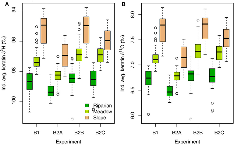
Figure 4. Boxplots of individual average keratin δ²H (A) and δ¹⁸O (B) values for each B experiment and nesting habitat.

Analysis of the model output suggests that 94–95% of H and O isotopic variation among B experiments, habitats, and individuals can be attributed to two variables: (1) body water turnover time, and (2) the proportion of water influx coming from drinking (p_Fdw; Figure 5, Supplementary Figure B1). Although neither variable was forced directly, both respond to differences in resource availability within the model framework, wherein individuals with greater access to water and higher drinking frequency ingest more drinking water, driving greater excretion of liquid waste and shorter turnover times.

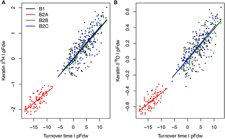
Figure 5. Partial linear regression relationships between individual average keratin δ²H (A) and δ¹⁸O (B) values (Y) and body water turnover time (X₁), given proportion of water influx coming from drinking (p_Fdw; X₂) for each B experiment. Relationships do not differ among experiments, but keratin absolute isotope values in B2A birds are more negative than in other B birds due to lower turnover rates, despite higher p_Fdw (Supplementary Figure B1). Multiple linear regression models are: for δ²H, Y = −97.41 + 0.12X₁ – 20.35X₂, R² = 0.95; for δ¹⁸O, Y = 6.78 + 0.04X₁ – 5.63X₂, R² = 0.94.

Environmental Variability

Between-habitat isotopic variation in environmental substrates in the E experiments produces a much wider range of modeled keratin δ²H and δ¹⁸O values than the behavioral/physiological effects modeled in the B experiments (e.g., >40‰ for H; Figures 4, 6). The relative pattern among birds nesting in different habitats is the same as that observed in the B experiments, but within- and between-habitat variability in keratin isotopic compositions is substantially higher for all the E experiments. The range of tissue isotope values is somewhat reduced in the E2A and E2C experiments, in which greater demand for resources and/or a larger search distance induce more vigorous and spatially dispersed foraging. In contrast, higher feeding success rates in the E2B experiment allow slope-nesters to focus their foraging more within the slope, and slightly increase the difference in mean values between this habitat and the others. Among-individual variability within nesting habitats is also much greater than in the B experiments, with the largest ranges for birds nesting in the slope (Figure 6).

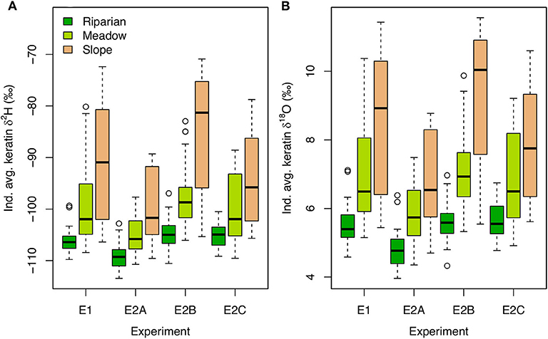
Figure 6. Boxplots of individual average keratin δ²H (A) and δ¹⁸O (B) values for each E experiment and nesting habitat.

Among-individual variation in mean input flux isotopic ratios is the dominant driver of variability in keratin isotopic compositions in the E experiments, with secondary influence of variation in turnover time and the proportion of water influx coming from drinking (Figure 7; Supplementary Figures B2, B3). Together, these variables explain 97% of H and O isotopic variation predicted across the E experiments. These results suggest that isotopic variability among habitats within a local environment, combined with selective utilization of habitats as discussed above, may produce substantial inter-individual isotopic variation in consumer tissues. The extent of this effect is sensitive to the behavioral characteristics of species and individuals, and is accentuated at the population level when individuals forage locally within isotopically distinct habitats. The extent of environmental heterogeneity, too, is predicted to be a strong determinant of inter-individual isotopic variability, within the extreme case of the B experiments (isotopically uniform environment) suggesting an order of magnitude-reduction in variability among individuals.

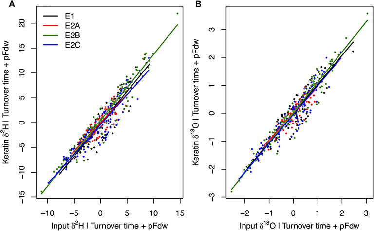
Figure 7. Partial linear regression relationships between individual average keratin δ²H (A) and δ¹⁸O (B) values (Y) and mean input flux isotope ratios (X₁), given body water turnover time (X₂) and proportion of water influx coming from drinking (X₃) for each E experiment. Relationships do not differ among experiments, and keratin absolute isotope values span similar ranges across behavioral properties due to factors producing offsets in isotopic relationships among experiments held constant here (but see Supplementary Figures B2, B3). Multiple linear regression models are: for δ²H, Y = 2.58 + 1.28X₁ + 0.10X₂ + 26.73X₃, R² = 0.97; for δ¹⁸O, Y = −5.17 + 1.05X₁ + 0.03X₂ + 19.26X₃, R² = 0.97.

Comparisons and Measured Data

Lastly, we compare simulated isotopic variation with variance observed in locally grown feathers from hatch-year Spotted Towhees in RBC. Measured feather δ²H values (mean ± SD) were −105.32 ± 12.97‰ (range = 59.32‰) and δ¹⁸O values were 13.1 ± 2.53‰ (range = 11.85‰; Supplementary Table B2). Results for the B experiments show much smaller variation in keratin δ²H and δ¹⁸O values than do either the E and E1B1 experiments or field-collected towhee data (Figure 8; Supplementary Table B2). Variation is more similar in the E and E1B1 experiments, implying that the among-individual physiological differences considered here accentuate the tissue isotopic variability imparted by environmental heterogeneity, but by a relatively small amount. These experiments approximate the variation in the observed samples well, meaning that the model toolbox reproduces observed within-site among-individual isotopic variance only when environmental isotopic variability is accounted for. Among the E experiments, between-individual variation is smallest in the E2A and E2C experiments (Figure 8). In the former case, that is likely because 16 slope-associated model individuals died, compressing variation toward ranges typical of the riparian and meadow habitats; in the latter, reduced variance is attributable to the larger foraging area of individuals.

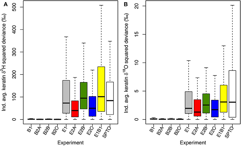
Figure 8. Boxplots of squared deviances (x_i – μ_x)² of individual average keratin δ²H (A) and δ¹⁸O (B) values from the mean values for each experiment. Squared differences are also shown for measured δ²H and δ¹⁸O data for locally grown feathers from Spotted Towhees (SPTO) in RBC. Model results reflect randomly assigned nesting locations, meaning that the probability of nesting in each habitat is proportional to the fraction of the landscape with that classification and the majority (mean = 89/105) of individuals nest in the slope habitat. Means, sample variances, SDs, and ranges for each experiment and data are reported in Supplementary Table B2.

Discussion

Within-site among-individual variation in consumer tissue H and O isotope ratios has been documented across a range of biological systems. Despite its critical importance for the use of these isotope systems in ecology, the drivers and characteristics of this variation are generally poorly understood (but see, e.g., Hobson et al., 2012). On one hand, differences in behavior and physiology might produce differences in the isotope mass-balance and biochemistry of individuals through mechanisms such as different metabolic rates, water loss pathways, or diet composition (Wolf and Martinez del Rio, 2000; Meehan et al., 2003; Smith and Dufty, 2005; Langin et al., 2007). On the other, individuals that forage within isotopically heterogeneous environments might access resources with different isotope ratios, contributing isotopic variation to their tissues (Meehan et al., 2003; Smith and Dufty, 2005; Hobson et al., 2012). Here we present the first model-based assessment of some of these mechanisms, evaluating whether, within the context of our current understanding, these different processes can replicate observed variability within a natural system.

We benchmark our model results against a new dataset of keratin H and O isotopic compositions for conspecific individual birds growing feathers at a common site. Datasets of this kind are valuable to quantify the magnitude of local among-individual isotopic variance and investigate the causes of such variance, but only a few datasets currently exist (e.g., for H: Meehan et al., 2003; Wunder et al., 2005; Langin et al., 2007; Hobson et al., 2012, 2014; for O: Hobson and Koehler, 2015). Our dataset provides further evidence of large within-site among-individual isotopic variance. Values of δ²H and δ¹⁸O for towhees span ~60 and >10‰ ranges, respectively. The δ²H range is far larger than that observed in American Redstarts (12–20‰; Langin et al., 2007), and more similar to those measured for shorebirds (60 and 113‰; Wunder et al., 2005; Rocque et al., 2006; but see Larson and Hobson, 2009) and raptors (~50‰; Meehan et al., 2003). Although ranges observed for towhees do not exceed variation in precipitation between breeding and non-breeding grounds for this species (Bowen et al., 2005b), the substantial local among-individual isotopic variance documented here would dramatically reduce the certainty and usefulness of assignment tests for this species.

The importance of heterogeneity in the isotopic compositions of environmental substrates as a control of within-population isotopic variance of animals has been proposed previously (Meehan et al., 2003; Smith and Dufty, 2005), but few studies have measured this environmental variability. Here we document substrate heterogeneity by sampling potential prey items. Even though our results are based on small numbers of pooled samples (see section Environmental Isoscape Models), ranges in prey water and organic matter isotope ratios within RBC are large, and among-habitat differences provide evidence for evaporation as the dominant underlying driver of observed patterns (Supplementary Figures A3, A6). Even though we did not measure spatial variability in drinking water directly, similar patterns are expected, assuming that any drinking water available in the non-riparian habitats comes from transient puddles and/or leaf-intercepted water subject to relatively large evaporative enrichments (Supplementary Figure A7). Given the environmental isotopic variability that we observed (or modeled, for drinking water), preferential use of resources from differing, isotopically distinct habitats within the study area could offer a plausible mechanism for the high variance observed in towhee feathers.

We test this idea using a mechanistic modeling framework and a range of different assumptions about environmental, behavioral, and physiological heterogeneity. The models do reproduce the magnitude of the observed isotopic variance in the towhee population, but are only able to do so when environmental isotopic variability is accounted for (E and E1B1 experiments; Figure 8; Supplementary Table B2). This suggests that variation in diet isotopic ratios may be a strong driver of variance within this population (Figure 7). Small differences exist between measured and predicted variance even in the E and E1B1 models, which could reflect the inappropriateness of some model assumptions. For example, we use data from hatch-year birds to ensure that our dataset only includes locally grown feathers. Hatch-year birds are often more isotopically variable than adults, which could be attributed to their limited access to drinking water (Meehan et al., 2003; Smith and Dufty, 2005; Langin et al., 2007), variable nest microclimate, habitat segregation between molting adults and hatch-year birds, and/or difference in feather growth rate. These factors may not be adequately reflected in the idealized model used here.

We find that behavioral and physiological differences among individuals, in this case largely driven by differences in local habitat quality, contribute more subtly to among-individual isotopic difference than does environmental isotopic heterogeneity. Habitat characteristics affect individual drinking and foraging behavior (Figure 3), body water balance, and tissue isotopic compositions (Figures 4, 5). In the model system this effect accentuates that of environmental isotopic variability in an isotopically heterogeneous environment. This prediction is consistent with the proposal that difference in body water balance might contribute to the inter-individual isotopic variability observed in local populations (Wolf and Martinez del Rio, 2000; Meehan et al., 2003; Smith and Dufty, 2005) but also with a previous model-based assessment suggesting that this contribution is likely to be relatively small (Magozzi et al., 2019).

These results are somewhat dependent on the range of parameter values tested. Although the ranges chosen here are generally consistent with observed data, where these are available (Goldstein, 1988), the values and variability of some parameters are poorly constrained. Comparison of the inter-individual variation expressed within our individual B experiments, where the prescribed range of trait values was relatively small, with the variation across experiments (where mean trait value differences were 5–10 times larger; Table 1), however, shows low values of behaviorally and physiologically driven isotopic variance relative to the E experiments in all cases.

Moreover, all of the physiological mechanisms that we have identified as potential drivers of significant isotopic variation, including inter-individual differences in foraging success and drinking and body water turnover, are in turn strongly forced by environmental heterogeneity. Thus, we suggest that environmental heterogeneity, whether via variation in substrate isotope ratios or behavioral and physiological correlates, may be the dominant, first-order control on inter-individual H and O isotope variance within consumer populations. For example, the high variance observed in our system relative to that observed by Langin et al. (2007) might in part reflect the influence of aridity and strongly contrasting evaporative effects among habitats in the RBC environment. Similarly, in coastal environments generalist species that use both terrestrial and marine resources might be more isotopically variable (Rocque et al., 2006; but see Larson and Hobson, 2009), particularly where individuals specialize their feeding within this context (Vander Zanden et al., 2010). High local among-individual isotopic variance might therefore be expected in habitats characterized by large environmental and isotopic heterogeneity, particularly those encompassing gradients (e.g., humidity, terrestrial to marine) along which the isotopic composition of environmental substrates and/or stressors affecting the body water balance of individuals vary extensively. In real-world settings, temporal environmental variability may act to enhance or reduce the effect of variation among habitats, depending on its scale and frequency. This first-order expectation represents a hypothesis to be tested with additional field-collected samples, and complexities associated with patterns of habitat use and specialization may strongly modulate or overwhelm differences in environmental variability for some systems. If our hypothesis is supported, however, it would suggest that uncertainty in isotope-based methods will generally be higher for species occupying environments characterized by larger isotopic and/or environmental heterogeneity, implying predictable differences in the utility of these methods for different groups of organisms, depending on the characteristics of their environment.

Our model, like any other, is clearly not comprehensive and other relevant mechanisms not considered here may also contribute to consumer H and O isotope variability. Potential factors may include changes in metabolic pathways (e.g., increased reliance on lipid metabolism; Estep and Hoering, 1980; Sessions et al., 1999) during exercise or starvation, and differences in dietary macronutrient composition (Meehan et al., 2003; Langin et al., 2007). Given this, we emphasize that our results represent predictions of isotopic patterns expected given a limited suite of environmental, physiological, and behavioral mechanisms and range of parameter space. The results appear to be reasonable and meaningful when tested against the towhee dataset, but future models should incorporate and explore additional mechanisms, evaluating their effects on isotopic variance and testing whether they are consistent across systems or system-specific.

Conclusions

In this work we introduce a modeling framework providing explicit predictions of the magnitude and patterns of isotopic variance in H and O among individual terrestrial endotherms (birds) living at a common site under different sets of assumptions. This set of tools offers new opportunities to explore and constrain the potential mechanisms giving rise to such variance. Particularly, we demonstrate that simulation model-based inference can successfully be used to understand the potential effects of multiple variance-generating processes on a measured variable (here isotopic composition of body tissues), offering a complementary approach to data-based inference. Within the model framework, isotopic heterogeneity in the local habitat emerges as the dominant driver of local among-individual isotopic variance, with its effect accentuated by differences in body water balance. If verified, this implies that among-individual variance in body tissue H and O isotopic compositions may be strongly linked to the degree of isotopic heterogeneity in local environmental H and O sources.

Future studies should investigate the movement and behavior of birds in natural environments and data should be used to adapt the model mechanisms to specific groups or taxa. For example, insectivorous birds might acquire most water from diet, which would dampen the effect from variable contribution of drinking water to the body water pool seen here. Similarly, the post-fledging movements of hatch-year birds are poorly known but the habitat used by adult birds during molt to a prebasic plumage before migration is believed to greatly influence the variance measured in feathers from unknown locations and such a shortcoming in our understanding would also deserve further investigation. Future work should also test additional mechanisms that might potentially modify the magnitude and patterns of such variation such as nutritional status and macronutrient composition, and assess the consistency of each effect across systems. The models developed here may be used to predict the usefulness of isotope-based applications for specific groups of organisms or environments and develop optimal, system-specific sampling strategies in ecology and forensic research. As greater confidence in model mechanisms and predictions develops, these models could also be ultimately applied to produce variance estimates to be used in statistical estimation of origin where measurements are inadequate to do so.

Data Availability Statement

Code to run the models and generate datasets used in this study can be found online (Bowen and Magozzi, 2020).

Ethics Statement

The animal study was reviewed and approved by University of Utah Institutional Animal Care and Use Committee (number 18-02002). Written informed consent was obtained from the owners for the participation of their animals in this study.

Author Contributions

SM and GB conceived ideas and designed methodology, with support from CT, HVZ, and MW. DP and PD analyzed the LiDAR data. JH and CS provided the feather samples. KP collected samples of environmental substrates and prepared substrate and feather samples for isotopic analyses. SM and GB led the writing of the manuscript. All authors contributed critically to the drafts and gave final approval for publication.

Funding

This work was supported by U.S. National Science Foundation Grants EF-1241286 and DBI-1565128.

Conflict of Interest

The authors declare that the research was conducted in the absence of any commercial or financial relationships that could be construed as a potential conflict of interest.

Acknowledgments

We wish to thank Jon Gale, Ahmed Bwika, Jason Socci, Evan Buechley, and Monte Neate-Clegg for their help in feather collection.

Supplementary Material

The Supplementary Material for this article can be found online at: https://www.frontiersin.org/articles/10.3389/fevo.2020.536109/full#supplementary-material

References

Ambrose, S. J., Bradshaw, S. D., Withers, P. C., and Murphy, D. P. (1996). Water and energy balance of captive and free-ranging Spinifexbirds (Eremiornis carteri) North (Aves:Sylviidae) on Barrow Island, Western Australia. Aust. J. Zool. 44, 107–117. doi: 10.1071/ZO9960107
Bowen, G. J. (2010). “Statistical and geostatistical mapping of precipitation water isotope ratios,” in Isoscapes, eds J. B. West, G. J. Bowen, T. E. Dawson, and K. P. Tu (Dordrecht: Springer), 139–160. doi: 10.1007/978-90-481-3354-3_7
Bowen, G. J., Chesson, L., Nielson, K., Cerling, T. E., and Ehleringer, J. R. (2005a). Treatment methods for the determination of δ2H and δ18O of hair keratin by continuous-flow isotope-ratio mass spectrometry. Rapid Commun. Mass Spectrom. 19, 2371–2378. doi: 10.1002/rcm.2069
Bowen, G. J., and Magozzi, S. (2020). Data From: Spatial-Lab/CombinedDynamicHOModel: Matilda (Version v0.2). Zenodo. Available online at: http://doi.org/10.5281/zenodo.4048720 (accessed September 24, 2020).
Bowen, G. J., and Revenaugh, J. (2003). Interpolating the isotopic composition of modern meteoric precipitation. Water Resour. Res. 39:1299. doi: 10.1029/2003WR002086
Bowen, G. J., Wassenaar, L. I., and Hobson, K. A. (2005b). Global application of stable hydrogen and oxygen isotopes to wildlife forensics. Oecologia 143, 337–348. doi: 10.1007/s00442-004-1813-y
Carpenter-Kling, T., Pistorius, P., Connan, M., Reisinger, R., Magozzi, S., and Trueman, C. N. (2019). Sensitivity of δ13C values of seabird tissues to combined spatial, temporal, and ecological drivers: a simulation approach. J. Exp. Mar. Biol. Ecol. 512, 12–21. doi: 10.1016/j.jembe.2018.12.007
Chamberlain, C. P., Blum, J. D., Holmes, R. T., Feng, X., Sherry, T. W., and Graves, G. R. (1996). The use of isotope tracers for identifying populations of migratory birds. Oecologia 109, 132–141. doi: 10.1007/s004420050067
Chesson, L. (2012). Calibration of Primary Laboratory Reference Materials FH, UH, ORX, and DS as well as Secondary Reference Material POW for Hydrogen, Carbon, Nitrogen, and Oxygen Stable Isotope Ratio Analysis. IsoForensics Report.
Clegg, S. M., Kelly, J. F., Kimura, M., and Smith, T. B. (2003). Combining genetic markers and stable isotopes to reveal population connectivity and migration patterns in a neotropical migrant, Wilson's Warbler (Wilsonia pusilla). Mol. Ecol. 12, 819–830. doi: 10.1046/j.1365-294X.2003.01757.x
Cooper, C. E., Withers, P. C., Hurley, L. L., and Griffith, S. C. (2019). The field metabolic rate, water turnover, and feeding and drinking behavior of a small avian desert granivore during a summer heatwave. Front. Physiol. 10:1405. doi: 10.3389/fphys.2019.01405
Craig, H. (1961). Isotopic variations in meteoric waters. Science 133:1702. doi: 10.1126/science.133.3465.1702
Ehleringer, J. R., Bowen, G. J., Chesson, L. A., West, A. G., Podlesak, D. W., and Cerling, T. E. (2008). Hydrogen and oxygen isotope ratios in human hair are related to geography. Proc. Natl. Acad. Sci. U.S.A. 105, 2788–2793. doi: 10.1073/pnas.0712228105
Estep, M. F., and Hoering, T. C. (1980). Biogeochemistry of the stable hydrogen isotopes. Geochim. Cosmochim. Acta 44, 1197–1206. doi: 10.1016/0016-7037(80)90073-3
Goldstein, D. L. (1988). Estimates of daily energy expenditure in birds: the time-energy budget as an integrator of laboratory and field studies. Am. Zool. 28, 829–844. doi: 10.1093/icb/28.3.829
Gomez, C., Guerrero, S., FitzGerald, A. M., Bayly, N. J., Hobson, K. A., and Cadena, C.-D. (2019). Range-wide populations of a long-distance migratory songbird converge during stopover in the tropics. Ecol. Monogr. 89:e01349. doi: 10.1002/ecm.1349
Gow, E. A., Stutchbury, B. J. M., Done, T., and Kyser, T. K. (2012). An examination of stable hydrogen isotope (δD) variation in adult and juvenile feathers from a migratory songbird. Can. J. Zool. 90, 585–594. doi: 10.1139/z2012-024
Haché, S., Hobson, K. A., Villard, M.-A., and Bayne, E. M. (2012). Assigning birds to geographic origin using feather hydrogen isotope ratios (δ2H): importance of year, age, and habitat. Can. J. Zool. 90, 722–728. doi: 10.1139/z2012-039
Hobson, K. A. (1999). Tracing origins and migration of wildlife using stable isotopes: a review. Oecologia 120, 314–326. doi: 10.1007/s004420050865
Hobson, K. A., Bowen, G. J., Wassenaar, L. I., Ferrand, Y., and Lormee, H. (2004). Using stable hydrogen and oxygen isotope measurements of feathers to infer geographical origins of migrating European birds. Ecosyst. Ecol. 141, 477–488. doi: 10.1007/s00442-004-1671-7
Hobson, K. A., Kardynal, K. J., and Koehler, G. (2019). Expanding the isotopic toolbox to track monarch butterfly (Danaus plexippus) origins and migration: on the utility of stable oxygen isotope (δ18O) measurements. Front. Ecol. Evol. 7:224. doi: 10.3389/fevo.2019.00224
Hobson, K. A., and Koehler, G. (2015). On the use of stable oxygen isotope (δ18O) measurements for tracking avian movements in North America. Ecol. Evol. 5, 799–806. doi: 10.1002/ece3.1383
Hobson, K. A., Van Wilgenburg, S. L., Faaborg, J., Toms, J. D., Rengifo, C., Sosa, A. L., et al. (2014). Connecting breeding and wintering grounds of neotropical migrant songbirds using stable hydrogen isotopes: a call for an isotopic atlas of migratory connectivity. J. Field Ornithol. 85, 237–257. doi: 10.1111/jofo.12065
Hobson, K. A., Van Wilgenburg, S. L., Wassenaar, L. I., and Larson, K. (2012). Linking hydrogen (δ2H) isotopes in feathers and precipitation: sources of variance and consequences for assignment to isoscapes. PLoS ONE 7:e35137. doi: 10.1371/journal.pone.0035137
Hobson, K. A., and Wassenaar, L. I. (1997). Linking brooding and wintering grounds of neotropical migrant songbirds using stable hydrogen isotopic analysis of feathers. Oecologia 109, 142–148. doi: 10.1007/s004420050068
Hobson, K. A., and Wassenaar, L. I. (2019). Tracking Animal Migration With Stable Isotopes, 2nd Edn. Amsterdam: Academic Press, 1–268. doi: 10.1016/B978-0-12-814723-8.00001-5
Kelly, J. F., Atudorei, V., Sharp, Z. D., and Finch, D. M. (2002). Insights into Wilson's Warbler migration from analyses of hydrogen stable isotope ratios. Oecologia 130, 216–221. doi: 10.1007/s004420100789
Kirkley, J. S., and Gessaman, J. A. (1990). Water economy of nestling Swainson's hawks. Condor 92, 29–44. doi: 10.2307/1368380
Langin, K. M., Reudink, M. W., Marra, P. P., Norris, D. R., Kyser, T. K., and Ratcliffe, L. M. (2007). Hydrogen isotopic variation in migratory bird tissues of known origin: implications for geographic assignment. Oecologia 152, 449–457. doi: 10.1007/s00442-007-0669-3
Larson, K. W., and Hobson, K. A. (2009). Assignment to breeding and wintering grounds using stable isotopes: a comment on lessons learned by Rocque et al. J. Ornithol. 150, 709–712. doi: 10.1007/s10336-009-0408-0
Magozzi, S., Vander Zanden, H. B., Wunder, M. B., and Bowen, G. J. (2019). Mechanistic model predicts tissue-environment relationships and trophic shifts in animal hydrogen and oxygen isotope ratios. Oecologia 191, 777–789. doi: 10.1007/s00442-019-04532-8
Marder, J., Withers, P. C., and Philpot, R. G. (2003). Patterns of cutaneous water evaporation by Australian pigeons. Isr. J. Zool. 49, 111–129. doi: 10.1560/68CG-H6AQ-PD4C-2PQ3
McKechnie, A. E., Wolf, B. O., and Martinez del Rio, C. (2004). Deuterium stable isotope ratio sas tracers of water resource use: an experimental test with rock doves. Oecologia 140, 191–200. doi: 10.1007/s00442-004-1564-9
Meehan, T. D., Rosenfield, R. N., Atudorei, V. N., Bielefeldt, J., Rosenfield, L. J., Stewart, A. C., et al. (2003). Variation in hydrogen stable-isotope ratios between adult and nestling Cooper's Hawks. Condor 105, 567–572. doi: 10.1093/condor/105.3.567
National Ecological Observatory Network (2017). Data Product DP3.30015.001, Ecosystem Structure. Boulder, CO: Battelle, NEON. Available online at: http://data.neonscience.org (accessed August 4, 2017).
Nordell, C. J., Haché, S., Bayne, E. M., Solymos, P., Foster, K. R., Godwin, C. M., et al. (2016). Within-site variation in feather stable hydrogen isotope (δ2Hf) values of boreal songbirds: implications for assignment to molt origin. PLoS ONE 12:e0172619. doi: 10.1371/journal.pone.0163957
Qi, H., Coplen, T. B., and Wassenaar, L. I. (2011). Improved online δ18O measurements of nitrogen- and sulfur-bearing organic materials and a proposed analytical protocol. Rapid Commun. Mass Spectrom. 25, 2049–2058. doi: 10.1002/rcm.5088
Reese, J. A., Tonra, C., Viverette, C., Marra, P. P., and Bulluck, L. P. (2018). Variation in stable hydrogen isotope values in a wetland-associated songbird. Waterbirds 41, 247–256. doi: 10.1675/063.041.0304
Rocque, D. A., Ben-David, M., Barry, R. P., and Winker, K. (2006). Assigning birds to wintering and breeding grounds using stable isotopes: lessons from two feather generations among three intercontinental migrants. J. Ornithol. 147, 395–404. doi: 10.1007/s10336-006-0068-2
Rubenstein, D. R., and Hobson, K. A. (2004). From birds to butterflies: animal movement patterns and stable isotopes. Trends Ecol. Evol. 19, 256–263. doi: 10.1016/j.tree.2004.03.017
Sakamoto, T., Komatsu, K., Shirai, K., Higuchi, T., Ishimura, T., Setou, T., et al. (2019). Combining microvolume isotope analysis and numerical simulation to reproduce fish migration history. Methods Ecol. Evol. 10, 59–69. doi: 10.1111/2041-210X.13098
Schoeller, D. A., Leitch, C. A., and Brown, C. (1986). Doubly labeled water method: in vivo oxygen and hydrogen isotope fractionation. Am. J. Physiol. 251, R1137–R1143. doi: 10.1152/ajpregu.1986.251.6.R1137
Sessions, A. L., Burgoyne, T. W., Schimmelmann, A., and Hayes, J. M. (1999). Fractionation of hydrogen isotopes in lipid biosynthesis. Org. Geochem. 30, 1193–1200. doi: 10.1016/S0146-6380(99)00094-7
Smit, B., and McKechnie, A. E. (2015). Water and energy fluxes during summer in an arid-zone passerine bird. Int. J. Avian Sci. 157, 774–786. doi: 10.1111/ibi.12284
Smith, A. D., and Dufty, A. M. (2005). Variation in the stable hydrogen isotope composition of Northern Goshawk feathers: relevance to the study of migration origins. Auk 107, 547–558. doi: 10.1093/condor/107.3.547
Smith, B. S., and Greenlaw, J. S. (2015). “Spotted Towhee (Pipilo maculatus), Version 2.0,” in The Birds of North America, ed P. G. Rodewald (Ithaca: Cornell Lab of Ornithology). doi: 10.2173/bna.263
Soetaert, K., Petzoldt, T., and Setzer, R. W. (2010). Solving differential equations in R: package deSolve. J. Stat. Softw. 33, 1–25. doi: 10.18637/jss.v033.i09
Soto, D. X., Kohler, G., Wassenaar, L. I., and Hobson, K. A. (2017). Re-evaluation of the hydrogen stable isotopic compositions of keratin calibration standards for wildlife and forensic science applications. Rapid Commun. Mass Spectrom. 31, 119–1203. doi: 10.1002/rcm.7893
Storm-Suke, A., Wassenaar, L. I., Nol, E., and Norris, D. R. (2012). The influence of metabolic rate on the contribution of stable-hydrogen and oxygen isotopes in drinking water to quail blood plasma and feathers. Funct. Ecol. 26, 1111–1119. doi: 10.1111/j.1365-2435.2012.02014.x
Studds, C. E., McFarland, K. P., Abury, Y., Rimmer, C. C., Hobson, K. A., Marra, P. P., et al. (2012). Stable-hydrogen isotope measures of natal dispersal reflect observed population declines in a threatened migratory songbird. Divers. Distrib. 18, 919–930. doi: 10.1111/j.1472-4642.2012.00931.x
Tieleman, B. I., and Williams, J. B. (2000). The adjustment of avian metabolic rates and water fluxes to desert environments. Physiol. Biochem. Zool. 73, 461–479. doi: 10.1086/317740
Trueman, C. N., Jackson, A. L., Chadwick, K. S., Coombs, E. J., Freyer, L. J., Magozzi, S., et al. (2019). Combining simulation modeling and stable isotope analyses to reconstruct the last known movements of one of nature giants. PeerJ. 7:e7912. doi: 10.7717/peerj.7912
Trueman, C. N., and St John Glew, K. (2019). “Isotopic tracking of marine animal movement,” in Tracking Animal Migration With Stable Isotopes, 2nd Edn, eds K. A. Hobson and L. I. Wassenaar (Amsterdam: Academic Press), 137–182. doi: 10.1016/B978-0-12-814723-8.00006-4
van Dijk, J. G. B., Meissner, W., and Klaassen, M. (2014). Improving provenance studies in migratory birds when using feather hydrogen stable isotopes. J. Avian Biol. 45, 103–108. doi: 10.1111/j.1600-048X.2013.00232.x
Vander Zanden, H. B., Biorndal, K. A., Reich, K. J., and Bolten, A. B. (2010). Individual specialists in a generalist population: results from a long-term stable isotope series. Biol. Lett. 6, 711–714. doi: 10.1098/rsbl.2010.0124
Wassenaar, L. I., and Hobson, K. A. (2003). Comparative equilibration and online technique for determination of non-exchangeable hydrogen of keratins for use in animal migration studies. Isotopes Environ. Health Stud. 39, 1–7. doi: 10.1080/1025601031000096781
Waterisotopes Database (2018). Query: South Latitude = 40.7770, North Latitude = 40.8000, West Longitude = −111.7725, East Longitude = −111.8060, Type = River or stream. Available online at: http://waterisotopesDB.org (accessed October 1, 2018).
Wolf, B. O., and Martinez del Rio, C. (2000). Use of saguaro fruit by white-winged doves: isotopic evidence of a tight ecological association. Oecologia 124, 536–543. doi: 10.1007/s004420000406
Wunder, M. B. (2010). “Using isoscapes to model probability surfaces for determining geographic origins,” in Isoscapes, eds J. B. West, G. J. Bowen, T. E. Dawson, and K. P. Tu (Dordrecht: Springer), 251–270. doi: 10.1007/978-90-481-3354-3_12
Keywords: agent-based, physiology, isoscape, models, mechanistic, isotopic variation, hydrogen, oxygen
Citation: Magozzi S, Vander Zanden HB, Wunder MB, Trueman CN, Pinney K, Peers D, Dennison PE, Horns JJ, Şekercioğlu ÇH and Bowen GJ (2020) Combining Models of Environment, Behavior, and Physiology to Predict Tissue Hydrogen and Oxygen Isotope Variance Among Individual Terrestrial Animals. Front. Ecol. Evol. 8:536109. doi: 10.3389/fevo.2020.536109
Received: 18 February 2020; Accepted: 18 November 2020;
Published: 11 December 2020.
Edited by:
John Whiteman, Old Dominion University, United StatesReviewed by:
Keith Alan Hobson, Western University, CanadaKevin McCluney, Bowling Green State University, United States
Copyright © 2020 Magozzi, Vander Zanden, Wunder, Trueman, Pinney, Peers, Dennison, Horns, Şekercioğlu and Bowen. This is an open-access article distributed under the terms of the Creative Commons Attribution License (CC BY). The use, distribution or reproduction in other forums is permitted, provided the original author(s) and the copyright owner(s) are credited and that the original publication in this journal is cited, in accordance with accepted academic practice. No use, distribution or reproduction is permitted which does not comply with these terms.
*Correspondence: Sarah Magozzi, sarah.magozzi@szn.it