


ABSTRACT
We present new, accurate predictions for rotational line positions, excitation energies, and transition probabilities of the 12C13C isotopologue Swan d3Π–a3Π system 0–0, 0−1, 0−2, 1−0, 1−1, 1−2, 2−0, 2−1, and 2−2 vibrational bands. The line positions and energy levels were predicted through new analyses of published laboratory data for the 12C13C lines. Transition probabilities were derived from recent computations of transition dipole moments and related quantities. The 12C13C line data were combined with similar data for 12C2, reported in a companion paper, and applied to produce synthetic spectra of carbon-rich metal-poor stars that have strong C2 Swan bands. The matches between synthesized and observed spectra were used to estimate band head positions for a few of the 12C13C vibrational bands and to verify that the new computed line data match observed spectra. The much weaker C2 lines of the bright red giant Arcturus were also synthesized in the band head regions.
Export citation and abstract BibTeX RIS
1. INTRODUCTION
Electronic spectra of C2 have been studied extensively, from the near-infrared to the far-ultraviolet, and the general properties of the various band systems have been known for some time (e.g., Huber & Herzberg 1979). Of the known C2 transitions, the Swan system (d3Πg–a3Πu) has been studied for more than a century. This system has been the focus of much attention mainly because of its presence in many astronomical objects including comets, interstellar clouds, late-type stars, and the Sun (Brooke et al. 2013 and references therein). The characteristic bands of the Swan system are also detected easily in hydrocarbon combustion.
In spite of much interest in the main isotopic form 12C2, only limited laboratory data are available for the minor isotopologues, 12C13C and 13C2. However, lines arising from 12C13C are seen in many carbon stars; therefore, accurate laboratory measurements are needed. In a previous study, Pesic et al. (1983) reported the observation of several bands of the Swan system at moderate resolution using a hollow cathode discharge of argon and 13C-enriched benzene. They carried out a rotational analysis of six 13C2 bands and the 0–1, 1–1, and 1–0 bands of 12C13C. The 13C2 bands were much stronger in their spectra, causing frequent overlapping with the rotational lines of 12C13C. Recently, several 12C2, 13C2, and 12C13C bands of the Swan system were observed at low resolution by Dong et al. (2013) during a carbon isotope analysis experiment with laser ablation of samples containing 12C and 13C mixtures. In a high-resolution study, Amiot (1983) recorded spectra of the 0–0 Swan bands of 12C2, 13C2, and 12C13C isotopologues using a Fourier transform spectrometer (FTS). High-resolution data on bands with higher vibrational levels, (v ⩾ 1), have been lacking, and so astronomers have been forced to use approximate line positions predicted from estimated 12C13C spectroscopic constants, which are entirely based on 12C2 spectroscopic constants and isotopic relationships.
In related work, Amiot & Verges (1982) reported an analysis of the 0–0 band of the Ballik–Ramsay system of 13C2 and 12C13C using high-resolution spectra recorded with an FTS. This study was followed with a high-resolution analysis of 12 bands of the Ballik–Ramsay system of 13C2 (with v' = 0–6, v'' = 0–3) and seven bands of 12C13C (with v' = 0–3, v'' = 0–2) by Islami & Amiot (1986).
Along with the major isotopologue, the minor 12C13C isotopologue has also been observed in diverse astronomical sources, and has been used to determine their 12C/13C isotopic ratios. For example, Krishna Swamy (1987) performed statistical thermodynamic calculations to compare with the moderately high-resolution observations of comet West by Lambert & Danks (1983). More recently, Rousselot et al. (2012) obtained the 12C/13C isotopic ratios of 85 ± 20 and 80 ± 20 for comet T7 (LINEAR) and comet Q4 (NEAT), respectively. Hema et al. (2012) investigated the high-resolution spectra of R Coronae Borealis stars and hydrogen-deficient carbon stars by synthesizing the 0–1, 0–0, and 1–0 bands of the Swan system for 12C2 and 12C13C.
The present work has been undertaken to predict more precise line positions of the 12C13C Swan system based on spectroscopic constants from the FTS measurements determined by Amiot and coworkers, cited above. The spectroscopic constants for v = 1 and 2 in the d3Π state were estimated using accurate v = 0 constants and 12C13C equilibrium constants, which were estimated from the equilibrium constants of the 12C2 Swan system (Brooke et al. 2013) and isotopic relationships. We then applied these line data to the spectra of a carbon-rich low-metallicity star and to the well-studied K giant Arcturus.
2. METHOD OF CALCULATION
The rotational line positions of the 0–0 band of the 12C13C Swan system d3Π–a3Π (Amiot 1983), and the 0−0, 1−0, 1−1, 2−0, 2−1, 3−1, and 3−2 bands of the Ballik–Ramsay system (b3Σ−–a3Π) (Amiot & Verges 1982; Islami & Amiot 1986) were fitted simultaneously using the pgopher program (Western 2010).6 In addition to new spectroscopic constants for the b3Σ− state, this fit provided the constants for the v = 0, 1, and 2 vibrational levels of the a3Π state and the v = 0 level of d3Π state. The Amiot group observed several perturbations in the two band systems. All of the lines affected by local perturbations were given lower weights in the fits and were expected to have a minimal effect on the isotopic relationships. Next, the equilibrium constants of the a3Π and d3Π states of 12C13C were calculated (Table 1) using the equilibrium constants of these states in 12C2 (Brooke et al. 2013) and the isotopic relationships: ωei = ρωe, ωexei = ρ2ωexe, ωeyei = ρ3ωeye, Bei = ρ2Be, αei = ρ3αe, γei = ρ4γe, Dei = ρ4De, βei = ρ5βe, pei = ρ2pe, qei = ρ4qe, where ρ = (μ/μi)(1/2).
Table 1. Equilibrium Constants (in cm−1) of the a3Π and d3Π States of 12C13C
| Constants | a3Π | d3Πa |
|---|---|---|
| ωe | 1609.3651(20) | 1753.6109 |
| ωexe | 11.21028(91) | 16.2191 |
| ωeye | ... | −0.2442 |
| Be | 1.5692827(67) | 1.687683 |
| αe | 0.015596(11) | 0.018477 |
| γe × 105 | −0.0000271(44) | −0.000133 |
Download table as: ASCIITypeset image
The predicted a3Π state equilibrium constants, ωe = 1609.3728 cm−1, ωexe = 11.2097 cm−1, Be = 1.56938 cm−1, αe = 0.01563 cm−1, and γe = −2.5234 × 10⁻⁵ cm−1 agreed well with the values of ωe = 1609.3651 (20) cm−1, ωexe = 11.21028(91) cm−1, Be = 1.5692827(67) cm−1, αe = 0.015596(11) cm−1, and γe = −2.71(44) × 10−5 cm−1 obtained from the present fit. The calculated values of spectroscopic constants of the v = 0, 1, and 2 levels of the 12C13C a3Π state, obtained using the equilibrium constants described above, also agreed well with the corresponding values obtained from our fit. Assuming that similar agreement exists for the d3Π state, we predicted the rotational constants for the v = 1 and 2 vibrational levels with respect to the d3Π v = 0 constants as determined from the least squares fit. The other constants, such as Av, ADv, ov, λv, etc., for the v = 1 and 2 levels were fixed with respect to their v = 0 values, following the trend found in the d3Π state of 12C2 (Brooke et al. 2013). Tables 2 and 3 provide the observed constants for v = 0 and the calculated values for v = 1 and 2 in the d3Π state, along with the spectroscopic constants of the a3Π and b3Σ− states of 12C13C. The line positions in the 1−0, 1−1, 2−1, and 2−2 bands of 12C13C d3Π–a3Π transition, predicted using the constants of Tables 2 and 3, are expected to be more reliable than those calculated entirely using the isotopic relationships. The inclusion of the 0−1, 1−1, and 1−0 line positions from Pesic et al. (1983) deteriorated the fit because of the large uncertainty in their measurements, which was partly due to strong overlapping from 13C2 bands.
Table 2. The Spectroscopic Constants of the a3Π and d3Π States of 12C13C
| Constantsa | a3Π | d3Π | ||||
|---|---|---|---|---|---|---|
| v = 0 | v = 1 | v = 2 | v = 0 | v = 1b | v = 2b | |
| Tv | 0.0 | 1586.94453(71) | 3151.4685(15) | 19377.1594(22) | 21097.3555 | 22781.8544 |
| Av | −15.27166(78) | −15.2584(11) | −15.2343(16) | −14.0130(43) | −13.9 | −13.85 |
| ADv × 104 | 1.956(30) | 1.93(30) | 1.59(31) | 3.93(36) | 3.93 | 3.93 |
| Bv | 1.5614782(40) | 1.5458286(43) | 1.5301249(49) | 1.6783998(93) | 1.6594194 | 1.6395154 |
| Dv × 106 | 5.92776(83) | 5.9380(13) | 5.9479(14) | 6.3418(84) | 6.5235 | 6.7052 |
| λv | −0.15368(64) | −0.15348(77) | −0.1528(14) | 0.0448(21) | 0.0448 | 0.0448 |
| ov | 0.67076(44) | 0.66805(49) | 0.66352(91) | 0.5907(22) | 0.595 | 0.597 |
| pv | 0.002226(25) | 0.002273(17) | 0.002461(26) | 0.003542(62) | 0.00354 | 0.00354 |
| qv × 104 | −4.8888(56) | −5.3670(84) | −6.003(18) | −6.634(15) | −6.65 | −6.67 |
Notes. aAdditional constants, H0 = 1.291(61) × 10−12, pD0 = −4.89(78) × 10−8, qD0 = 1.769(14) × 10−8, H1 = 9.9(21) × 10−13, qD1 = 2.268(32) × 10−8, qD2 = 3.055(85) × 10−8 for the a3Π state and H0 = 1.55(22) × 10−11 for the d3Π state were also determined. bFixed values; see text for details.
Download table as: ASCIITypeset image
Table 3. The Spectroscopic Constants of the b3Σ− State of 12C13C
| Constants | v = 0 | v = 1 | v = 2 | v = 3 |
|---|---|---|---|---|
| Tv | 5635.15027(57) | 7055.49421(47) | 8454.52008(67) | 9832.2947(13) |
| Bv | 1.4331269(40) | 1.4177524(40) | 1.4023565(41) | 1.3869552(47) |
| Dv × 106 | 5.71904(72) | 5.72882(72) | 5.73592(77) | 5.7448(13) |
| γv × 103 | −1.507(175) | −1.514(174) | −1.577(174) | −1.543(175) |
| λv | 0.15067(72) | 0.15294(56) | 0.15341(69) | 0.15715(95) |
Download table as: ASCIITypeset image
3. CALCULATION OF LINE STRENGTHS
The line strengths for various bands of the d3Π–a3Π transition of 12C13C were calculated in the form of Einstein A-coefficients and oscillator strengths (f-values). Computational details for the 12C2 Swan bands are provided by Brooke et al. (2013). The Einstein A-coefficients have been calculated using the following equation:
where  is the rotational line strength factor (the Hönl–London factor),
  is the transition wavenumber (cm−1),
  is the transition dipole moment (TDM) in debye, and Einstein A values are in s−1.
The potentials of the two electronic states were calculated using the RKR program (Le Roy 2004),7 with the equilibrium constants of the two electronic states of 12C13C (Table 1). The RKR potentials of the upper and lower states and the TDM function,  (from high-level ab initio calculations), are then employed in the LEVEL program (Le Roy 2007)8 to calculate the wave functions, ψv, J. We used the TDM functions provided by Schmidt & Bacskay (2007) and Kokkin et al. (2007) in our line strength calculation. The TDM matrix elements obtained from LEVEL for each band are then used in pgopher (Western 2010) for the calculation of Einstein A-values. The Einstein A-values are converted into oscillator strengths (f-values) using the following equation:
Complete data for the 12C13C Swan band 0−1, 0−2, 1−0, 1−1, 1−2, 2−0, 2−1, and 2−2 band transitions considered in this study are given in Table 4. The quantities include: vibrational and rotational line designations, observed and calculated wavenumbers and their differences, energy levels, Einstein A values and oscillator strengths (f-values), and summary line designations.
Table 4. Assignments, Wavenumbers, Excitation Energies, and Transition Probabilities of Individual 12C13C Transitionsa
| Assignments | Wavenumbers | Lower E. | Einstein A | f-value | Transition | |||||||||
|---|---|---|---|---|---|---|---|---|---|---|---|---|---|---|
| v' | v'' | J' | J'' | F' | F'' | p' | p'' | Observed | Calculated | Residual | ||||
| (cm−1) | (cm−1) | (cm−1) | (cm−1) | (s−1) | ||||||||||
| 0 | 0 | 2 | 3 | 1 | 1 | e | e | ... | 19370.7339 | ... | −1.9280 | 2.617529E+06 | 7.470145E−03 | pP1e(3) |
| 0 | 0 | 3 | 4 | 1 | 1 | e | e | ... | 19368.3875 | ... | 8.9471 | 3.359125E+06 | 1.044125E−02 | pP1e(4) |
| 0 | 0 | 4 | 5 | 1 | 1 | e | e | ... | 19366.1767 | ... | 22.6651 | 3.647616E+06 | 1.192968E−02 | pP1e(5) |
| 0 | 0 | 5 | 6 | 1 | 1 | e | e | ... | 19364.1266 | ... | 39.2790 | 3.777913E+06 | 1.278095E−02 | pP1e(6) |
| 0 | 0 | 6 | 7 | 1 | 1 | e | e | ... | 19362.2592 | ... | 58.8343 | 3.841279E+06 | 1.331293E−02 | pP1e(7) |
| 0 | 0 | 7 | 8 | 1 | 1 | e | e | ... | 19360.5916 | ... | 81.3680 | 3.872963E+06 | 1.366804E−02 | pP1e(8) |
| 0 | 0 | 8 | 9 | 1 | 1 | e | e | 19359.147 | 19359.1360 | 0.0110 | 106.9088 | 3.888559E+06 | 1.391776E−02 | pP1e(9) |
| 0 | 0 | 9 | 10 | 1 | 1 | e | e | ... | 19357.9005 | ... | 135.4790 | 3.895607E+06 | 1.410102E−02 | pP1e(10) |
| 0 | 0 | 10 | 11 | 1 | 1 | e | e | ... | 19356.8905 | ... | 167.0950 | 3.897993E+06 | 1.424030E−02 | pP1e(11) |
| 0 | 0 | 11 | 12 | 1 | 1 | e | e | ... | 19356.1098 | ... | 201.7693 | 3.897814E+06 | 1.434929E−02 | pP1e(12) |
Notes. av = vibrational q.n., J = rotational q.n., F = spin component, p = parity, lower E. = Lower energy level.
Only a portion of this table is shown here to demonstrate its form and content. A machine-readable version of the full table is available.
Download table as: DataTypeset image
4. APPLICATION OF THE NEW C2 DATA TO STELLAR SPECTRA
4.1. Generation of Line Lists
In stellar abundance analyses, one needs line lists with wavelengths, lower-state excitation energies, and transition probabilities (usually expressed as log gf values) for all relevant molecular and atomic absorbers. For C2, we generated a line list suitable for input to the current version of the LTE synthetic spectrum code, MOOG (Sneden 1973). The relevant quantities for each line were derived for 12C2 from the data in the table in Appendix A of Brooke et al. (2013) and for 12C13C from the data in Table 4. The resultant line list, containing nearly 184,000 transitions, can be obtained from the authors.9
Wavenumbers in air were computed from the vacuum wavenumbers with the Birch & Downs (1994) corrected version of Edlén's (1966) conversion formula, and inverted to produce air wavelengths in Angstroms. For lines with laboratory detections we adopted the measured wavenumbers, and used the predicted wavenumbers for the other transitions. We changed the lower-state energies E'' from units of cm−1 to eV, a common convention in astronomy. Finally, we converted the Einstein spontaneous emission coefficient A' to the commonly used gf via

The MOOG code follows the development of Schadee (1964) for diatomic molecules. His approach combined Saha and Boltzmann equations to form a transition lower-state electron number density in terms of the constituent atomic free number densities (after molecular equilibrium computations), their partition functions, and the molecular dissociation energy.
The C2 dissociation energy is well determined (e.g., D0 = 6.30 eV, Urdahl et al. 1991; 6.27 eV, Pradhan et al. 1994). We adopted D0 = 6.27 eV. In the Sun, and most cool stars, the free number density of carbon depends almost entirely on the CO formation, that is

where P(C) is the fictitious (in the absence of any molecular or ionized species) pressure of carbon. The C2 molecule is at most a trace constituent in typical, cool, stellar atmospheres, so its dissociation energy is unimportant for this equilibrium equation. In line-forming regions (τ ∼ −1) of the solar atmosphere, C2 comprises about 0.01% of the total carbon, and in lower-pressure G–K giants the percentage of C2 is orders of magnitude less.
Diatomic molecular partition functions mathematically cancel out in the Schadee (1964) line opacity equations. However, the partition functions for homonuclear 12C2 and heteronuclear 12C13C differ by a factor of two because the parent molecule has half as many energy states as the isotopic form. This difference cannot be accounted for in MOOG's implementation of the Schadee formalism (D. L. Lambert 2013, private communication; see also the discussion in Cohen et al. 2006). Since C2 is the only homonuclear molecule of interest in stellar spectroscopic investigations, we chose to make no general alteration to the synthesis code. Rather, like Cohen et al., we simply divided the gf values computed as above by a factor of two to mimic the partition function differences. This choice is reflected in our final C2 line list, which contains all parent and isotopic lines from this study.
4.2. C2 Swan Bands in Carbon-enhanced Metal-poor Stars
The major absorption bands of the C2 Swan system occur in the 4500–5700 Å spectral region. However, in stars with abundance mixes like that of the Sun, the Swan system produces relatively weak absorption features that often are significantly contaminated with or completely masked by atomic lines. The strongest Swan bands, those of the Δv = 0 sequence, occur near 5100 Å, just where the strongest MgH A2Π–X2Σ+ bands are located (e.g., Hinkle et al. 2013 and references therein). Indeed, Swan system lines often serve as contaminants to MgH. As such, they increase the difficulty in deriving reliable Mg isotopic ratios from MgH, while not presenting enough isolated C2 features for a reliable carbon abundance analysis. In order to make a cleaner test of our new line list, first we decided to generate synthetic spectra of the Swan bands to compare with high-resolution spectra of so-called "carbon-enhanced metal-poor" stars (CEMP; see Beers & Christlieb 2005).
Cohen et al. (2006) conducted a high-resolution spectroscopic survey of 15 CEMP stars. Their spectra, obtained with the HIRES instrument, are available in the Keck Observatory archive. The observations were made as part of the program, "The first generation of stars in the Galaxy" (PI: J. Cohen), on 2002 September 27 and 28. Five 1200 s exposures were collected, using a 0 86 slit width, which yields a spectral resolution of R ≈ 45,000. Spectra cover the range between 3840 and 5330 Å. For more details about the observations, the interested reader is referred to Cohen et al. These archival spectra were reduced using the MAKEE10 spectrum reduction package, then continuum-normalized and shifted to rest-frame using IRAF.11
All of the CEMP stars in the Cohen et al. (2006) survey are very metal-poor (–3.30 ⩽ [Fe/H] ⩽ −1.85), relatively warm (4945 K ⩽ Teff ⩽ 6240 K) subgiants and giants (2.0 ⩽ log g ⩽ 3.7). These parameters combine to yield very weak atomic absorption lines in their spectra. However, the majority of CEMP stars are also enriched in neutron-capture (n-capture) elements, most noticeably in barium (Z = 56), the lanthanides (57 ⩽ Z ⩽ 71), and lead (Z = 82). Transitions arising from ionized n-capture species can be seen especially in the blue–violet spectral regions. Detailed abundance studies of these kinds of CEMP stars indicate that the dominant n-capture synthesis mechanism has been the slow "s-process" (e.g., Sneden et al. 2008 and references therein), so such stars are labeled CEMP-s.
Almost all very metal-poor halo stars have relative overabundances with respect to iron of the "α" elements Mg, Si, Ca, and Ti. The Cohen et al. (2006) sample is no exception, with 〈[Mg/Fe]〉 ∼ +0.5, but since the mean metallicity of their stars is 〈[Fe/H]〉 ∼ −2.1, the total magnesium abundance is still very small, thus absorption by MgH must be very weak or completely absent. Of course, carbon is very overabundant in CEMP stars; the mean enhancement in the Cohen et al. sample is 〈[C/Fe]〉 ∼ 1.9 (〈[C/H]〉 ∼ −0.2), making C2 the dominant spectral feature near 5000 Å.
We inspected our set of Cohen et al. (2006) data, seeking stars with the largest C2 absorption combined with the lowest 12C/13C ratios, in order to see the 12C13C isotopic band structures. We found clearly identifiable 1–0 and 2–1 P-branch band heads of this isotopologue in six stars, and 0–1 band heads in one star. For the 0–1 band region we added a spectrum of the CEMP subgiant, LP 625–44 (Aoki et al. 2006 and references therein), which was obtained by David Lai with Hamspec at Lick Observatory. From these spectra, we estimated the observed band head wavelength differences, λ(12C13C)–λ(12C2). For this exercise, we defined the wavelength of deepest absorption to be the band head, which we estimated to be ∼0.3 Å blueward of the P-branch red–edge wavelength. From the wavelength differences, we computed 12C13C band head wavelengths using the corresponding 12C2 wavelengths derived by Brooke et al. (2013). In Table 5 we list the 12C2 band heads from that paper, our observed stellar and predicted 12C13C band heads, our predicted isotopic shifts, and those of Pesic et al. (1983). Clearly, our predicted band head positions are in good agreement with the observed ones.
Table 5. Calculated and Observed Band Head Positions of 12C13C and Comparison of Isotope Shifts
| Band | 12C2 | 12C13C | 12C2–12C13C Isotope Shift | |||||||
|---|---|---|---|---|---|---|---|---|---|---|
| Brooke et al. (2013) | Observeda | Predicteda | Predicteda | Pesic et al. (1983) | ||||||
| (cm−1) | (Å) | (cm−1) | (Å) | (cm−1) | (Å) | (cm−1) | (Å) | (cm−1) | (Å) | |
| (0–1)b | 17739.75 | 5635.492 | 17770.1 | 5625.9 | 17770.28 | 5625.810 | −30.53 | 9.682 | −30.40 | 9.641 |
| (1–2) | 17898.58 | 5585.483 | ... | ... | 17925.74 | 5577.020 | −27.16 | 8.463 | −27.07 | 8.438 |
| (0–0) | 19354.79 | 5165.240 | ... | ... | 19354.40 | 5165.344 | 0.39 | −0.104 | 0.52 | −0.139 |
| (1–1) | 19490.23 | 5129.345 | ... | ... | 19487.80 | 5129.985 | 2.43 | −0.640 | 2.42 | −0.637 |
| (2–2) | 19611.01 | 5097.754 | ... | ... | 19608.07 | 5098.519 | 2.94 | −0.764 | 4.03 | −1.045 |
| (1–0)b | 21104.15 | 4737.079 | 21071.0 | 4744.6 | 21070.54 | 4744.635 | 33.61 | −7.556 | 34.08 | −7.667 |
| (2–1) | 21201.72 | 4715.278 | 21167.2 | 4723.0 | 21167.52 | 4722.897 | 34.20 | −7.619 | 34.14 | −7.607 |
Notes. aThis paper; band head positions and isotope shifts are given in wavenumbers (cm−1) as well as in Angstrom units in air. bIsotope shifts (in Å and cm−1 units) observed by Dong et al. (2013) are 9.7 Å, −30.58 cm−1 for the 0–1 band and −7.5 Å, 33.35 cm−1 for the 1–0 bands.
Download table as: ASCIITypeset image
We chose to concentrate on the star HE 0212–0557 to compare our predicted 12C13C line data with observations over larger wavelength ranges. For details about the model parameter and abundance determinations of this star, see Cohen et al. (2006). Briefly, they derived Teff = 5075 K, log g = 2.15, vmicro = 1.8 km s−1, and metallicity = [Fe/H] = −2.27. They reported abundances for 18 other elements. Highlights for our purposes are: [C/Fe] = 1.74, 12C/13C = 3–4, [α-element/Fe] = [〈Mg i, Ca i, Ti i, Ti ii〉/Fe] = +0.2, and [rare-earth-elements/Fe] = [〈Ba ii, La ii, Ce ii, Pr ii, Nd ii〉/Fe] = +2.2. The enormous overabundances of carbon and the rare-earth neutron-capture abundances definitely assign HE 0212–0557 to the CEMP-s category.
We first produced synthetic spectra with the MOOG code, generating input quantities as follows. A model atmosphere for HE 0212–0557 with the Cohen et al. (2006) parameters Teff, log g, [Fe/H], vmicro was calculated by interpolating in the ATLAS model grid (Kurucz 2011 and references therein).12 We constructed the line lists beginning with the 12C2 and 12C13C lines described above, and added atomic lines from Kurucz's line compendium.13 For most atomic lines, we adopted the transition probabilities from the Kurucz database, but for neutron-capture elements (particularly the rare-earth ions) we adopted the gf's determined in a series of papers by the Wisconsin atomic physics group (Sneden et al. 2009 and references therein). The computed spectra were then convolved with Gaussian functions that empirically accounted for the combined effects of the Keck spectrograph slit function and stellar macroturbulence. Finally, we compared the synthetic spectra to the observed HE 0212–0557 spectrum, which had been corrected for its apparent radial velocity and continuum-normalized.
Some illustrative spectra of 12C2 and 12C13C bands in HE 0212–0557 are provided in Figures 1 and 2. We show spectra for small wavelength ranges that include the 0–0 and 1–1 band heads in Figure 1. Absorption by C2 dominates the spectrum blueward of 5165 Å. Isotopic wavelength shifts of the Δv = 0 bands are very small; the 12C2 and 12C13C band heads are indistinguishable. Nevertheless, it is easy to see that the observed spectrum must include large contributions from 12C13C lines. We varied the carbon isotopic ratio and the total carbon abundance until the best synthetic/observed spectrum match was achieved, deriving log ε(C) = 8.12 ± 0.05 ([C/Fe] = 1.8) and 12C/13C ≈ 4–5. Both of these results are in excellent accord with those of Cohen et al. (2006).
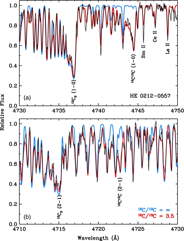
Figure 1. Observed and synthetic spectra for HE 0212–0557 around the 0–0 and 1–1 Swan system band heads. In each panel the black line is the observed spectrum. The blue line represents a synthesis with only 12C2 lines: 12C/13C = ∞. The red line represents a synthesis with substantial 12C13C contributions: 12C/13C = 3.5. In panel (a) the 0–0 band head is shown, along with a small additional region to the red, without strong C2 lines. Two Mg i b lines are labeled in the panel. In panel (b) the 1–1 band head is shown. Atomic lines are included in the syntheses, but their absorptions are overwhelmed by those of the C2 lines. Download figure: Figure 2. Observed and synthetic spectra for HE 0212–0557 around the 2–1 and 1–0 Swan system band heads. The line colors are the same as in Figure 1. Some of the atomic lines included in the syntheses have noticeable absorption. In panel (a) a few prominent rare-earth element transitions are labeled. In panel (b) note that there are many individual 1–0 transitions mixed in the 2–1 12C2 and 12C13C band head lines. Download figure:
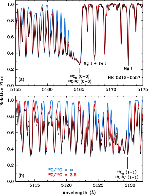
Panel (a) of Figure 1 also includes a 10 Å region redward of the 0–0 band head, which is almost devoid of C2 absorption. Several prominent features here are due to Fe i, but there are also two of the three Mg i b lines, which are labeled in the figure. In solar abundance mixtures the Mg i lines dominate the 5160–5190 Å spectral region. Their relative weakness compared to C2 is one of the defining characteristics of an extreme CEMP star; HE 0212–0557 is a near-textbook example of such an object.
In Figure 2 we show small wavelength sections that cover the 1–0 and 2–1 band heads. Happily, the isotope shifts for the Δv = +1 sequence are large; the 12C13C band heads are about 8 Å to the red of their 12C2 counterparts. This allows a much easier estimation of the isotopic ratio. Our derived total carbon abundance (log ε(C) = 8.09 ± 0.05) and 12C/13C ratio (4.5 ± 0.5) are indistinguishable from those obtained from the Δv = 0 bands. In panel (a) of this figure we have labeled three prominent rare-earth, ionized-species transitions. These lines would be extremely weak in metal-poor stars without the enormous overabundances of the n-capture elements of HE 0212–0557. There are other n-capture absorptions that appear among the C2 bands; their inclusion in our syntheses improves the quality of the match to the observed spectrum. In panel (b) the 12C2 2–1 band head is easily identified since it dominates the absorption in the 4712–4716 Å region. One can also find the 12C13C 2–1 band head at 4722 Å, but this task is made much more difficult by the strong absorption lines in this region due to 1–0 12C2 and 12C13C.
Our stated errors for [C/Fe] and 12C/13C simply reflect uncertainties in matching the observed spectrum. Strong C2 Swan absorption occurs throughout the 4500–5200 Å region in HE 0212–0557. This makes accurate continuum placement somewhat difficult, especially near the C2 band heads. However, our synthetic spectra were computed over about 100 Å each in the Δv = 0 and +1 wavelength regions, and we derived consistent carbon abundances and isotopic ratios in all of the synthesized regions. Note that our ±0.05 error in total carbon abundance is very small because of the great sensitivity of the "double-metal" C2 absorption to the carbon abundance. In these illustrative synthetic spectrum computations, we have not attempted to estimate the effects of model atmosphere parameters on [C/Fe]; see Cohen et al. (2006) for an extensive uncertainty analysis. However, we should re-emphasize statements from many past isotopic investigations: derived 12C/13C ratios are almost totally insensitive to errors in Teff, log g, and [M/H] because the molecular parameters (dissociation and excitation energies, transition probabilities) are nearly identical for 12C2 and 12C13C.
Our HE 0212–0557 spectrum does not extend into the wavelength region of the Δv = −1 bands, which cover about 5400–5640 Å; the 12C2 0–1 band head lies at 5635 Å. These bands are somewhat weaker than the Δv = 0 and +1 sequences, and the isotopic shifts are to the blue. For example, the 12C13C 0–1 band head lies at 5625 Å. We synthesized this region to compare with the spectrum of another Cohen et al. (2006) star, HE 1150–0428, which has a very low 12C/13C ratio. We detected the 12C13C band head, and confirmed that our line list accurately matches the wavelengths of the observed spectrum. We concur with the Cohen et al. derived abundances ([C/Fe] ≈ +2.4 for [Fe/H] ≈ −3.3, and 12C/13C ≈ 4) in HE 0212–0557, but have no new information to add on the Δv = −1 band sequence.
4.3. C2 in Arcturus
The very bright K-giant star Arcturus has been studied at high spectral resolution for decades. The atmospheric parameters of this mildly metal-poor star are well known (Teff = 4300 K, log g = 1.50, vmicro = 1.5, [Fe/H] = −0.50; e.g., Bergemann et al. 2012). Its spectrum is used as a template for studies of other cool stars, which sometimes become differential analyses with respect to Arcturus.
The C2 Swan bands are very weak in the Arcturus spectrum, and their lines are often completely masked by strong atomic lines. Additionally, in discussing new line data for the MgH molecule, Hinkle et al. (2013) included an estimate of the Mg isotopic fractions in Arcturus. Thus, unlike the CEMP-s star discussed in Section 4.2, the MgH lines mixed in with the C2 Δv = 0 system in Arcturus make a carbon abundance analysis very challenging.
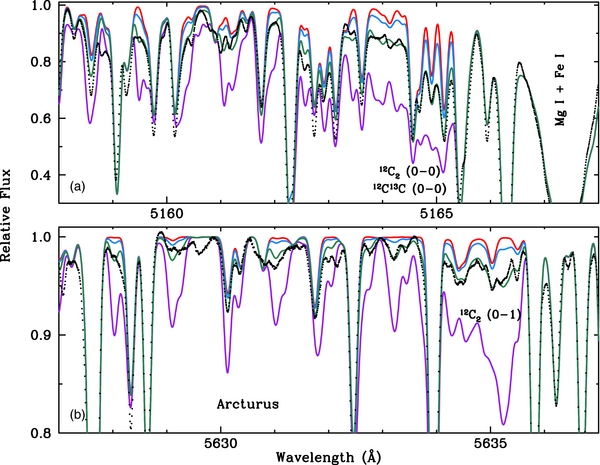
In Figure 3 we show synthesized and observed 0–0 and 0–1 Swan band heads in Arcturus. The observed spectrum is the very high resolution and signal-to-noise Arcturus atlas of Hinkle et al. (2000). The synthetic spectra were generated in the same manner as those of HE 0212–0557 discussed in Section 4.2. Both band heads are severely compromised with contamination by other species. In panel (a), the combined 12C2 and 12C13C 0–0 band head near 5165.3 Å is detectable, but obviously there are cleaner C2 features away from the band head that are better carbon abundance indicators. In panel (b), the much weaker 12C2 0–1 band head near 5636.5 Å is adequate for abundance studies because the atomic contamination is weak. However, we do not show the 12C13C band head near 5625.9 Å because it is completely buried underneath several strong atomic lines. Given the overall metallicity of Arcturus, 13C would need to be much more abundant to be detectable with confidence in this spectral region. Even less promising are the 12C2 and 12C13C 0–1 band heads at 4737 and 4744 Å; both are very weak and severely blended in the Arcturus spectrum. The best options for determining the carbon abundance from C2 in this star (and others like it) appear to be individual transitions of the 0–0 band and the 0–1 band head. The 12C/13C ratios in ordinary cool giants are probably better determined from other molecular features, e.g., the CN red system.
Figure 3. Observed and synthesized spectra of the 0–0 and 0–1 Swan band heads of 12C2 and 12C13C in K-giant star Arcturus. The black dots represent the observed spectrum. The green line shows the synthesis with the best fit to the observations. The blue and purple lines represent carbon abundances reduced and increased with respect to the best fit by factors of two. The red line is a synthetic spectrum with no contribution from C2. Download figure:
We thank David Lambert for very helpful discussions about molecular partition functions and David Lai for sharing his spectrum of LP 625–44 with us. This work is supported in part by NSF Grant AST-1211585 to C.S. and S.L. acknowledges partial support from PRIN INAF 2011. The paper was completed while C.S. was on a University of Texas Faculty Research Assignment in residence at the Department of Astronomy and Space Sciences of Ege University. Financial support from the University of Texas and The Scientific and Technological Research Council of Turkey (TÜBITAK, project No. 112T929) are greatly appreciated. The research at the University of York has been supported by funds from the Leverhulme Trust (UK). Some funding was also provided by the NASA laboratory astrophysics program.
The stellar spectra data presented herein were obtained at the W. M. Keck Observatory, which is operated as a scientific partnership among the California Institute of Technology, the University of California, and the National Aeronautics and Space Administration. The Observatory was made possible by the generous financial support of the W. M. Keck Foundation.
Footnotes
- 6
- 7
- 8
- 9
- 10
Software package developed by T. A. Barlow for reduction of Keck HIRES data. Available on the Keck Observatory home page, http://www.keckobservatory.org.
- 11
IRAF is distributed by the National Optical Astronomy Observatory, which is operated by the Association of Universities for Research in Astronomy, Inc., under cooperative agreement with the National Science Foundation.
- 12
- 13