


Abstract
This letter exploits the radial alignment between the Parker Solar Probe and BepiColombo in late 2022 February, when both spacecraft were within Mercury's orbit. This allows the study of the turbulent evolution, namely, the change in spectral and intermittency properties, of the same plasma parcel during its expansion from 0.11 to 0.33 au, a still unexplored region. The observational analysis of the solar wind turbulent features at the two different evolution stages is complemented by a theoretical description based on the turbulence transport model equations for nearly incompressible magnetohydrodynamics. The results provide strong evidence that the solar wind turbulence already undergoes significant evolution at distances less than 0.3 au from the Sun, which can be satisfactorily explained as due to evolving slab fluctuations. This work represents a step forward in understanding the processes that control the transition from weak to strong turbulence in the solar wind and in properly modeling the heliosphere.
Export citation and abstract BibTeX RIS

Original content from this work may be used under the terms of the Creative Commons Attribution 4.0 licence. Any further distribution of this work must maintain attribution to the author(s) and the title of the work, journal citation and DOI.
1. Introduction
The solar wind is a continuous stream of plasma particles released from the solar corona, the upper atmosphere of the Sun. It expands radially into interplanetary space, creating the heliosphere, the Sun-influenced region that extends far beyond Pluto's orbit. Along with this plasma flow, the Sun also generates a large-scale magnetic field, which is carried outward by the solar wind, pervading the whole heliosphere (Hundhausen 1972). At large distances from the Sun (i.e., >0.3 au), the solar wind can be reasonably considered to be in a state of fully developed turbulence. Fluctuations in the magnetic field, as well as in the plasma parameters, are indeed observed over a wide range of scales (Bruno & Carbone 2013). Additionally, their spectral (Coleman 1968) and intermittency (Sorriso-Valvo et al. 1999) properties suggest that the solar wind flow is at a high Reynolds number (Sorriso-Valvo et al. 1999; Parashar et al. 2019). Moreover, frequent observations of linear scaling of the mixed third-order moments of the fluctuations (Politano & Pouquet 1998) suggest that a well-developed magnetohydrodynamic (MHD) turbulent cascade is present (Sorriso-Valvo et al. 2007). The evolution of turbulence in the solar wind during its outward expansion is a central topic in heliophysics. Significant advances have been made over the past decades in observations, theory, and numerical simulations of solar wind turbulence (see the exhaustive review by Bruno & Carbone 2013). Nevertheless, there is still no complete, satisfactory description of solar wind turbulence evolution, namely, how and where turbulence is generated; how solar wind expansion, nonlinear interactions, and/or other mechanisms, such as plasma instabilities, collude in driving its development; and at what distance from the Sun turbulence reaches, in its spectral properties, the well-known flavor described by Kolmogorov (1941).
The radial evolution of solar wind turbulence is mostly studied using broad ensembles of measurements taken at different times and heliocentric distances and under different solar wind and solar conditions (Alberti et al. 2020; Chen et al. 2020). Due to the intrinsic variability and inhomogeneity of the solar wind and its solar sources, this approach cannot capture the basic evolution of waves, turbulence, and heating and their interaction with structures and transients, necessary for understanding the general processes and correctly modeling the heliosphere. With the launch in the 1970s of the two Helios spacecraft, which first probed the inner heliosphere as close as 0.3 au (Tu & Marsch 1995), it was possible to sample the same high-speed plasma flow (from the same coronal source region) at three different distances from the Sun in successive solar rotations. This allowed, for the first time, the study of the actual radial evolution of solar wind turbulence from 0.29 to 0.87 au (Bavassano et al. 1981, 1982a, 1982b; Perrone et al. 2019a, 2019b).
Unfortunately, since the success of the Helios mission, no other probes have been launched into the inner heliosphere, with the exception of the planetary missions to Mercury and Venus, MErcury Surface, Space ENvironment, GEochemistry and Ranging (MESSENGER) and Venus Express, neither specifically designed to study the solar wind and in fact almost continuously immersed in the planets' magnetospheres. This greatly limited the study of the evolution of the solar wind and its associated MHD properties. The only studies of solar wind turbulence evolution based on joint measurements by MESSENGER and near-Earth space observatories are due to Bruno & Trenchi (2014), Bruno et al. (2014), and Telloni et al. (2015).
In 2018, NASA launched the Parker Solar Probe (PSP; Fox et al. 2016), a mission designed to explore magnetic, electric, and velocity fields in the solar wind, making the closest approaches to the Sun ever made by a spacecraft. Two years later, with the launch of ESA-NASA's Solar Orbiter (SolO; Müller et al. 2020), the closest-to-the-Sun mission to provide both in situ and remote-sensing instrumentation (Zouganelis et al. 2020), an exciting and unprecedented opportunity to map the inner heliosphere opened up by exploiting the joint measurements of PSP and SolO along their complementary orbits (Velli et al. 2020). In particular, using specific configurations to obtain rare measurements of the same plasma parcel by the two radially aligned spacecraft can provide insight into the actual evolution of waves, turbulence, and heating under different conditions. The first PSP–SolO alignment was explored by Telloni et al. (2021a), who found that turbulence evolves from a less to a fully developed state as the solar wind expands from 0.1 to 1 au.
Although tailored to study Mercury's environment, the ESA's BepiColombo (BC; Benkhoff et al. 2010) mission, launched in 2018, provides interesting opportunities during its cruise phase to study the solar wind. Extensive preliminary investigations by Hadid et al. (2021) identified several configurations between BC and other space observatories useful for such studies. Alberti et al. (2022) studied the radial alignment between PSP orbiting at 0.17 au and BC at 0.6 au to investigate the evolution of the solar wind scaling features. They found that the nonlinear energy cascade becomes more efficient as the solar wind expands.
The two case studies by Telloni et al. (2021a) and Alberti et al. (2022) are limited, however, in that they do not allow the study of the evolution of near-Sun turbulence and thus the pristine solar wind, since they are based on radial alignments whose second probe is at least more than half the Earth–Sun distance away. Nor, for the aforementioned reasons, it is helpful in this regard to use all of the in situ measurements acquired by PSP at different distances during its orbits around the Sun, since these refer to highly inhomogeneous plasma streams, thus precluding an accurate investigation of the evolution of solar wind turbulence. A radial alignment between two of the three current inner heliospheric missions (i.e., PSP, SolO, and BC) at distances as close as 0.3–0.4 au would thus be crucial to investigate the evolution (if any) of solar wind turbulence in a still unexplored region, namely, within Mercury's orbit.
On 2022 February 23, PSP and BC were radially aligned. Their close distance to the Sun, 0.11 and 0.33 au, respectively, makes it possible to address the question of how similar or different this region is compared to the many detailed Helios studies just beyond that. This is the aim of the present work. Specifically, based on the in situ measurements gathered from both spacecraft, a thorough investigation of the evolution of the turbulent properties of the same plasma parcel as it moves away from the Sun is carried out from both an observational and a modeling perspective. The layout of this letter is as follows. Data analysis of PSP and BC data is given in Section 2, while Section 3 deals with the theoretical description of the turbulence evolution based on the nearly incompressible (NI) MHD model provided by Zank et al. (2017).
2. Data Analysis
Following Telloni et al. (2021a) and Alberti et al. (2022), the intervals at PSP and BC corresponding to the same plasma parcel were identified by requiring that, during the time the solar wind takes to cover the PSP–BC distance, BC covered the longitude separation it had from PSP when the plasma struck it (refer to the sketch of Figure 1 in Telloni et al. 2021a). The underlying assumption is that the speed of the solar wind, measured by the SPAN-Ai top-hat electrostatic analyzer of the Solar Wind Electrons Alphas & Protons suite (SWEAP; Kasper et al. 2016) on board PSP, is constant during its propagation to BC. Although impossible to fully corroborate (given the lack of BC plasma data), this ballistic assumption is reasonable based on the most recent observational and modeling studies carried out during the first SolO–PSP quadrature (Telloni et al. 2021b; Adhikari et al. 2022a; Biondo et al. 2022; Telloni et al. 2022a ), which show that the plasma flow reaches a steady-state speed at about 0.1 au from the Sun. Using this technique and assumption, it turns out that the plasma crossing PSP on 2022 February 24 from 04:15 to 05:37 UT impinged BC 1.23 days later, on 2022 February 25, at 09:48–11:10 UT. According to Panasenco et al. (2020) and Telloni et al. (2021a), the accuracy of the intervals so identified was checked by verifying that they were magnetically connected to the same source region at the Sun, namely, the equatorial extension of the same negative south coronal hole (Figure 1(a)). The orbits of the two probes in the 10 day period centered on the time of their radial alignment are shown, in side and top views of the equatorial plane, in Figures 1(b) and (c); PSP (red) and BC (blue) were orbiting near 0.11 and 0.33 au, respectively.
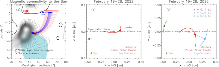
Figure 1. (a) Locations of PSP (blue) and BC (red) projected onto the solar wind source region (circles) and source surface (crosses) during the selected time intervals. Both spacecraft sample plasma from the same open magnetic field region with negative polarity (azure), below the neutral line (thick black curve). (b)–(c) Trajectories of PSP (red) and BC (blue) in the XZ and XY planes of the heliocentric inertial (HCI) coordinate system from 2022 February 19 to 28. Mercury's orbit (green) is also displayed for reference. Color-coded dots refer to the time of the PSP–BC lineup (marked by a dotted line); the corresponding PSP, BC, and Mercury distances from the Sun are reported in panel (c).
Download figure:
Standard image High-resolution imageThe solar wind plasma sampled by PSP and BC during their lineup belongs to a low-speed relatively quiescent flow (Malaspina et al. 2020; Dudok de Wit et al. 2020) with nearly constant velocity (309 km s−1) and density (600 cm−3) as measured by PSP, free of switchbacks (Kasper et al. 2019; Bale et al. 2019; Telloni et al. 2022b) and fairly well aligned with the (inward) magnetic field. This is clear from Figure 2, which displays the magnetic field data acquired by the fluxgate magnetometers on board PSP (FIELDS; Bale et al. 2016) and the BC Mercury Planetary Orbiter (Glassmeier et al. 2010; Heyner et al. 2021), rotated in the radial tangential normal (RTN) spacecraft-centered reference system and finally averaged at 1 minute resolution. Specifically, Figure 2 spans a time period of half a day centered on the radial alignment period (delimited by dashed vertical lines) and shows the components and magnitude of the magnetic field vector
B
(top panels) and its angle with the radial  (bottom panels) at PSP and BC distances from the Sun (left and right panels, respectively).
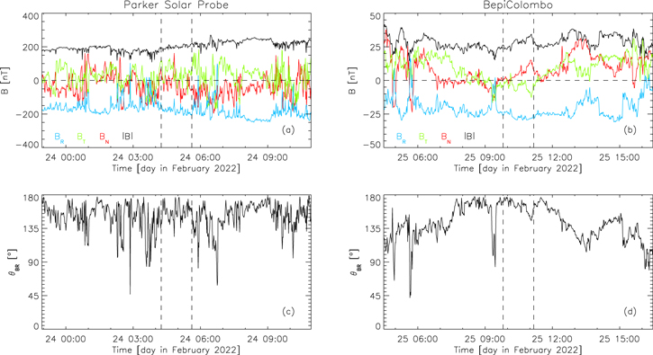
Figure 2. Magnetic field RTN components and magnitude (top) and inclination θRB of B with respect to the radial direction (bottom) as measured by PSP (left) and BC (right) at 0.11 and 0.33 au from the Sun. The dashed vertical lines mark the intervals corresponding to the same plasma parcel sampled by PSP and BC during their radial alignment.
Download figure:
Standard image High-resolution imageIn order to discuss in some detail the uncertainties associated with the determination of flow conjunction, how a 10% uncertainty in plasma velocity affects the identification of intervals tentatively corresponding to the same plasma parcel was studied. Assuming a solar wind speed 10% lower than that effectively measured by PSP, the orbital study would indicate that the same plasma parcel would cross PSP and BC on February 24 at 05:55 and February 25 at 15:04, respectively. On the other hand, if the flow velocity were 10% larger, then the two probes would be aligned on February 24 at 04:13 and February 25 at 06:51. In both cases, although the direction of the magnetic field would continue to be sunward at both PSP and BC, its orientation would be very different at the two distances from the Sun (Figures 2(c) and (d)). Specifically, while at PSP, the field would remain highly aligned with the plasma flow (θRB ∼ 180°), and at BC, the direction of the magnetic field would be oblique to the flow (θRB < 135°). Bearing in mind that the in situ measurements during the selected intervals at PSP and BC should exhibit the same large-scale magnetic field patterns (i.e., the same magnetic field direction and orientation with respect to the flow), this suggests a misalignment of the probes and, conversely, supports the correctness of the interval identification based on the actual wind speed measurements by PSP (further confirmed by the connectivity study), for which PSP and BC observations both correspond to a highly field-aligned flow with minor deviations from the radial. It is, however, worth noting that the magnetic field at BC continues to be radial about 2 hr before and 1 hr after the interval selected in the present work (this corresponds to a velocity about 5% higher and 2% lower than that measured by PSP). Therefore, to account for these uncertainties in the identification of the same plasma parcel and ensure statistical convergence, all of the following calculations and theoretical estimates were also carried out in extended intervals of 4.37 hr (still corresponding to plasma coming from the same source region; see Figure 1(a)). The results fully confirm those obtained in the 1.37 hr intervals selected with the orbital analysis.
At first glance, in the two intervals, the mean field is approximately radial and directed sunward. The amplitude of magnetic fluctuations is larger at PSP and decreases at BC, likely because of the evolution of turbulence and, specifically, the depletion of Alfvénic fluctuations during solar wind expansion. The dominant radial component appears to be roughly stationary and homogeneous, while some large-scale gradients are present in the plane perpendicular to the radial direction.
The study of the turbulence properties of the same solar wind plasma at the two different evolution stages is accomplished by assessing the spectral characteristics, compressibility, and intermittency of the magnetic field fluctuations observed at PSP and BC. The analysis is carried out at frequencies of ∼5 and 1 Hz for PSP and BC data, respectively. The spectrum of the magnetic field vector fluctuations δ
B
2, magnetic compressibility C = δ
B2/δ
B
2 (where δ
B2 is the power spectrum of the magnetic magnitude fluctuations), and flatness  (where Δ
B
are scale-dependent magnetic field vector increments and 〈〉 indicates ensemble average) are displayed from left to right (in red and blue for PSP and BC data, respectively) in Figure 3. Magnetic compressibility C and flatness
(where Δ
B
are scale-dependent magnetic field vector increments and 〈〉 indicates ensemble average) are displayed from left to right (in red and blue for PSP and BC data, respectively) in Figure 3. Magnetic compressibility C and flatness  are typically used proxies of Alfvénicity and intermittency. Here C is the ratio of the power associated with the fluctuations in magnetic magnitude δ
B2 and vector orientation δ
B
2 (which includes both directional and intensity fluctuations, so that δ
B
2 ≥ δ
B2). As such, C ∼ 1 (C ≪ 1) indicates a predominance of compressive (noncompressive) fluctuations in the solar wind (Bavassano et al. 1982a). Intermittency (a key ingredient of turbulence) affects the distribution functions of a fluctuating field by causing them to become gradually more peaked as smaller scales are involved (see Bruno & Carbone 2013). As a measure of the peakedness of a distribution (e.g., Frisch 1995; Dudok de Wit et al. 2013), the faster
are typically used proxies of Alfvénicity and intermittency. Here C is the ratio of the power associated with the fluctuations in magnetic magnitude δ
B2 and vector orientation δ
B
2 (which includes both directional and intensity fluctuations, so that δ
B
2 ≥ δ
B2). As such, C ∼ 1 (C ≪ 1) indicates a predominance of compressive (noncompressive) fluctuations in the solar wind (Bavassano et al. 1982a). Intermittency (a key ingredient of turbulence) affects the distribution functions of a fluctuating field by causing them to become gradually more peaked as smaller scales are involved (see Bruno & Carbone 2013). As a measure of the peakedness of a distribution (e.g., Frisch 1995; Dudok de Wit et al. 2013), the faster  grows continually at smaller scales (higher frequencies), the more intermittent the solar wind fluctuations are. The solar wind fluctuations primarily comprise two ingredients: Alfvénic fluctuations and a hierarchy of coherent structures (see discussion in Bruno et al. 2003). The former are propagating, noncompressive, stochastic fluctuations; as such, they tend to reduce magnetic compressibility and intermittency. The latter are compressive fluctuations generated by nonlinear interactions and are advected by the wind; as such, because of their coherent nature, they tend to increase magnetic compressibility and intermittency. It follows that the relative role of these two main components, and especially their evolution as the wind expands, can be assessed by the (opposite) effects they have on C and
  measured at different distances from the Sun (i.e., at different stages of turbulence evolution).
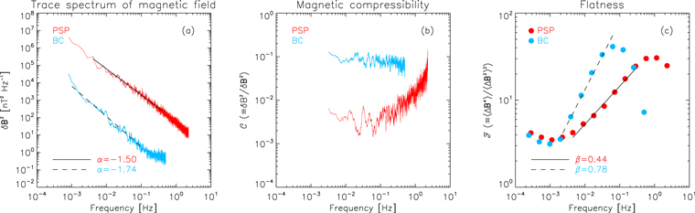
Figure 3. Magnetic spectral density δ
B
2 (a), magnetic compressibility C (b), and flatness  (c) at PSP (red) and BC (blue). Power-law fits to δ
B
2 and
(c) at PSP (red) and BC (blue). Power-law fits to δ
B
2 and  are superposed in the inertial range, and the spectral indexes α and β are given.
Download figure:
Standard image High-resolution imageThe trace spectra of magnetic field fluctuations at both PSP and BC distances exhibit a clear power-law scaling (Figure 3(a)), which covers at least two decades of frequencies in the inertial range. 34 However, while at PSP, the spectral index α = 3/2 is indicative of an Iroshnikov–Kraichnan (IK) picture of turbulence (Iroshnikov 1963; Kraichnan 1965), the steeper spectrum at BC (α ∼ 5/3) is suggestive of typical Kolmogorov turbulence (Kolmogorov 1941). The evolution from an IK-like to a Kolmogorov-like spectrum has already been observed in the inner heliosphere analyzing PSP measurements along its orbits around the Sun (Alberti et al. 2020; Chen et al. 2020). However, in those works, the transition region was estimated at larger heliocentric distances (≳0.5 and ∼0.4 au, respectively). The difference with respect to the present work, showing that the transition has already occurred at 0.3 au, may depend on the fact that Chen et al. (2020) and Alberti et al. (2020) analyzed different plasma streams sampled at different times. The variability of the plasma conditions could hide the fine details of the turbulence evolution in a specific plasma volume, which is instead accurately captured in the PSP–BC radial alignment studied here. Additionally, both magnetic compressibility and flatness increase moving away from the Sun (Figures 3(b) and (c), respectively), indicating a depletion of Alfvénic fluctuations during the wind expansion that causes coherent structures (likely strengthened further on by stream–stream dynamical interaction) to emerge more clearly and enhance intermittency (Bruno et al. 2003; Zank et al. 2020). The above results point to a clear evolution from weak, Alfvénic, less intermittent turbulence to strong, fully developed, highly intermittent turbulence as the wind expands from 0.11 to 0.33 au. Such an evolution had already been observed over a distance of 1 au from the Sun by Telloni et al. (2021a) exploiting the PSP–SolO radial alignment in 2020 September, but this work shows, for the first time, that turbulence evolution occurs at distances much closer to the Sun, specifically within Mercury's orbit (i.e., ≲0.3 au). This finding is also in agreement with the statistical study carried out by Alberti et al. (2020) during PSP's first two encounters with the Sun.
The observed turbulence evolution suggests that some processes are at work in governing the topology of solar wind fluctuations when moving away from the Sun. Likely candidates are enhancement of nonlinear interactions (Bruno & Carbone 2013; Zank et al. 2020), decrease in the imbalance between outward and inward Alfvén modes (Dobrowolny et al. 1980; Chen et al. 2020), velocity shears (Zank et al. 2017; Shi et al. 2020), and parametric instability (Malara & Velli 1996). To at least partially disentangle the above possible control parameters and complement the data analysis discussed in this section, the evolution of some turbulent properties is modeled in the next section with the NI MHD turbulence equations and compared with the observed results.
3. NI MHD Modeling
The Runge–Kutta fourth-order method is used to numerically solve the coupled 1D steady-state solar wind + NI MHD turbulence transport model equations of Adhikari et al. (2022c) from 0.11 to 0.33 au. Table 1 shows the boundary conditions at 0.11 au as obtained from PSP measurements, which, referring to an interval 1 hr and 22 minutes long, approximately correspond to the energy-containing range. The solar wind flow sampled by PSP (and BC) is aligned with the magnetic field (Figures 2(c) and (d)), which implies the observation of mostly slab/Alfvénic fluctuations (according to Zank et al. 2020). Therefore, the turbulence quantities measured at PSP correspond to the slab component (Bieber et al. 1996; Adhikari et al. 2020, 2022c; Zank et al. 2022). Accordingly, the boundary conditions for slab turbulence at 0.11 au are obtained from PSP measurements. The boundary conditions for 2D turbulence are instead obtained by assuming that the 2D turbulence energy (correlation length) is twice as large (small) as the corresponding value for slab turbulence 35 (Osman & Horbury 2007; Weygand et al. 2009; Adhikari et al. 2022c).
Table 1. Boundary Values at 0.11 au for Solar Wind Parameters (Speed U, Proton Density np
, Proton Temperature Tp
, and Electron Temperature Te
) and Turbulence Quantities (Outward and Inward Elsässer Energies  and the Corresponding Correlation Lengths λ± and Residual Energy ED
and the Corresponding Correlation Length λD
)
and the Corresponding Correlation Lengths λ± and Residual Energy ED
and the Corresponding Correlation Length λD
)
| Parameters | Values | Parameters | Values | Parameters | Values |
|---|---|---|---|---|---|
| U (km s−1) | 309 |
 (km2 s−2) (km2 s−2) | 18,000 |
 (km2 s−2) (km2 s−2) | 9000 |
| np (cm−3) | 600 |
 (km2 s−2) (km2 s−2) | 1476 |
 (km2 s−2) (km2 s−2) | 738 |
| Tp (K) | 400,000 |
 (km) (km) | 15,150 |
 (km) (km) | 30,300 |
| Te (K) | 320,000 |
 (km) (km) | 13,650 |
 (km) (km) | 27,300 |
 (km2 s−2) (km2 s−2) | −3663 |
 (km2 s−2) (km2 s−2) | −1832 | ||
 (km) (km) | 33,000 |
 (km) (km) | 66,000 |
Note. The superscript " ∞ " and asterisks denote the 2D and slab component, respectively.
Download table as: ASCIITypeset image
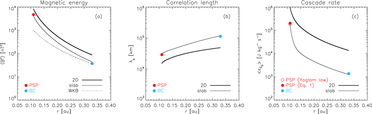
From left to right, Figure 4 displays the radial evolution of modeled transverse fluctuating magnetic energy 〈B2〉, the correlation length of the magnetic field fluctuations λb
, and the turbulent magnetic energy cascade rate  for 2D (thick curves) and slab (thin curves) turbulence. The theoretical values are compared with observations from PSP (red dots) and BC (blue dots) at 0.11 and 0.33 au, respectively.
Figure 4. Comparison between the theoretical and observed fluctuating magnetic energy (a), correlation length of the magnetic field fluctuations (b), and turbulent magnetic energy cascade rate (c) as a function of radial distance. Thick (thin) curves denote the 2D (slab) turbulence component. Red (blue) dots refer to PSP (BC) measurements. The dotted line in panel (a) marks the r−3 scaling predicted by the WKB assumption. The red filled and open dots in panel (c) refer to the  estimate from Equation (1) and the Yaglom law, respectively.
Download figure:
Standard image High-resolution image
As described by Adhikari et al. (2022c), the fluctuating magnetic field is first decomposed into perpendicular and parallel components in order to calculate the transverse fluctuating magnetic energy and the corresponding correlation length for the 2D and slab turbulence. In particular, λb at PSP and BC is estimated from the lag time corresponding to 1/e of autocorrelation at zero lag, which is then converted into the lag distance on the basis of the Taylor hypothesis (as mentioned before, assuming steady-state propagation of the solar wind, the same speed of 309 km s−1 measured at PSP is also considered at BC). The comparison of the theoretical slab 〈B2〉 with the observed values at PSP and BC clearly indicates that the evolution of the measured magnetic energy can be satisfactorily modeled by slab turbulence. As expected based on the boundary conditions, the theoretical 2D fluctuating magnetic energy is larger than the slab component. On the other hand, the relative radial profiles are quite similar. Interestingly, both the theoretical (2D and slab) and observed transverse fluctuating magnetic energy decrease more rapidly than the Wentzel–Kramers–Brillouin (WKB) prediction of r−3 (Zank et al. 1996; dotted line in Figure 4(a)). In addition, the theoretical slab correlation length of the magnetic field fluctuations is also consistent with observations (Figure 4(b)).
The observed fluctuating magnetic energy density cascade rate at PSP and BC is estimated as (Adhikari et al. 2021)

where Eb
= 〈B2〉/(μ0
ρ) (where μ0 and ρ are the magnetic permeability and proton mass density, respectively) is the fluctuating magnetic energy density, CK
= 1.6 is the Kolmogorov constant (inferred in numerical simulations from the height of the plateau in the compensated 3D energy spectrum at small Kolmogorov-scaled wavenumbers; e.g., Yeung & Zhou 1997), and kinj is the injection wavenumber for an ∼27 day solar rotation period (Adhikari et al. 2017). At the BC position, the proton density of np
= 67 cm−3 inferred by scaling the measurement at PSP as r−2 is used. The cascade rate of the theoretical 2D and slab fluctuating magnetic energy is instead derived using Equations (1)–(4) of Adhikari et al. (2022b), which are derived based on NI MHD turbulence transport theory (Zank et al. 2017). Observed  at both PSP and BC locations are very well modeled by the theoretical evolution of the slab magnetic energy density cascade rate. The energy transfer rate at the PSP position can also be directly estimated through the mixed third-order moment of the scale-dependent fluctuations (Yaglom law; Sorriso-Valvo et al. 2007) from PSP plasma and magnetic field data. Using the basic isotropic MHD formulation, the measured transfer rate is
  = 183 ± 22 kJ kg−1 s−1, consistent with previous observations at comparable distances (Hernández et al. 2021; Zhao et al. 2022b). This value, shown in Figure 4(c) as a red open dot, is in excellent agreement with the estimate by Equation (1) (red filled dot). Incidentally, such an energy transfer rate would result in a heating rate of ∼105 K proton–1 hr–1, a value consistent with the observed nonadiabatic solar wind cooling (Vasquez et al. 2007).
The striking agreement between the observations and the corresponding theoretical slab quantities strongly suggests that the turbulence evolution of the same plasma parcel at closer distances than Mercury's orbit can be successfully described by the NI MHD theory. From this model, it is possible to evaluate the cascade timescale  at both the PSP and BC orbits, obtaining
  and
and  s. Since the transport timescale
  s is shorter than the average cascade timescale, the evidence of clear spectral evolution indicates that the nonlinear dynamics has to be governed by 2D wavevectors in the above model (as it is by construction) and is possibly slowing down. Indeed, the spectral evolution is compatible with the freezing of the spectral index to a value of 5/3 reported in numerical simulations of MHD turbulence that include expansion (Grappin et al. 2022). In their work, spectral index evolution stops because the eddy turnover time increases as the expansion time, so the age of turbulence no longer changes with distance. Interestingly, the eddy turnover time is built on wavevectors transverse to the radial, which for this interval coincides with the 2D wavevectors; thus, independently of the model adopted, it seems that the evolution of turbulence in the inner heliosphere is determined by wavevectors transverse to the radial direction. This does not rule out the possibility that other processes (such as those mentioned in Section 1) may play an important role in the evolution of turbulence (possibly even at larger distances), but it provides a clear indication that, for the solar wind stream studied in the present paper, the NI MHD theory can itself explain how and where turbulence evolves in the very inner heliosphere, de facto addressing the question that motivated the present work.
D.T. was partially supported by the Italian Space Agency (ASI) under contract 2018-30-HH.0. B.S.-C. acknowledges support through STFC Ernest Rutherford Fellowship ST/V004115/1 and STFC grants ST/V000209/1 and ST/W00089X/1. L.S.-V. was funded by SNSA grants 86/20 and 145/18. L.A., L.-L.Z., and G.P.Z. acknowledge the partial support of NASA Parker Solar Probe contract SV4-84017, NSF EPSCoR RII-Track-1 cooperative agreement OIA-1655280, and a NASA IMAP grant through SUB000313/80GSFC19C0027. D.V. is supported by STFC Ernest Rutherford Fellowship ST/P003826/1 and STFC consolidated grants ST/S000240/1 and ST/W001004/1. A.M. and T.A. acknowledge the support from ASI-SERENA contract 2018-8-HH.O and ESA contract RFP/NC/IPL-PSS/JD/258.2016. Y.N. is supported by the Austrian Research Promotion Agency (FFG) under contract 865967. D.H. is supported by the German Ministerium für Wirtschaft und Energie and the German Zentrum für Luft- und Raumfahrt under contract 50QW1501. H.-U.A. is supported by the German Ministerium für Wirtschaft und Energie and the German Zentrum für Luft- und Raumfahrt under contracts 50OW2101 and 50QJ1501. The FIELDS and SWEAP teams acknowledge support from NASA contract NNN06AA01C.
Footnotes
- 34
The two-decade range of fluid scales where power-law fits were performed shifts to lower frequencies in the spacecraft frame moving from PSP to BC, in accordance with the well-known behavior of the inertial range to move to lower frequencies with increasing heliocentric distance (Telloni et al. 2015). It is also worth noting that the flattening of the BC spectrum at frequencies higher than about 0.1–0.2 Hz is due to the noise floor.
- 35