Quantum Gravity: A Fluctuating Point of View
 Jan M. Pawlowski1,2
  Manuel Reichert3,4*
- 1Institut für Theoretische Physik, Universität Heidelberg, Heidelberg, Germany
- 2xtreMe Matter Institute EMMI, GSI Helmholtzzentrum für Schwerionenforschung mbH, Darmstadt, Germany
- 3CP3-Origins, University of Southern Denmark, Odense, Denmark
- 4Department of Physics and Astronomy, University of Sussex, Brighton, United Kingdom
In this contribution, we discuss the asymptotic safety scenario for quantum gravity with a functional renormalization group approach that disentangles dynamical metric fluctuations from the background metric. We review the state of the art in pure gravity and general gravity–matter systems. This includes the discussion of results on the existence and properties of the asymptotically safe ultraviolet fixed point, full ultraviolet-infrared trajectories with classical gravity in the infrared, and the curvature dependence of couplings also in gravity–matter systems. The results in gravity–matter systems concern the ultraviolet stability of the fixed point and the dominance of gravity fluctuations in minimally coupled gravity–matter systems. Furthermore, we discuss important physics properties such as locality of the theory, diffeomorphism invariance, background independence, unitarity, and access to observables, as well as open challenges.
1 Introduction
One of the major challenges in theoretical physics is the unification of the standard model of particle physics (SM) with quantum gravity. Based on the classical Einstein–Hilbert action, gravity is perturbatively nonrenormalizable and hence cannot be expanded about a vanishing gravitational coupling, the Newton coupling. A very promising way out has been proposed by Weinberg [1], the asymptotic safety scenario. It draws from the theory of critical phenomena developed for investigating the phase structure of condensed matter and statistical systems. In the language of critical phenomena, the standard perturbation theory about a vanishing Newton coupling is an expansion about the free, Gaußian fixed point of the theory and fails since this fixed point is ultraviolet (UV)-repulsive in the relevant couplings. In turn, the asymptotic safety scenario builds upon the conjecture that quantum gravity also exhibits a nontrivial UV fixed point, the Reuter fixed point. This asymptotically safe fixed point should exhibit a finite-dimensional critical hypersurface, which renders the theory finite and predictive even beyond the Planck scale.
The method of choice for respective investigations is the renormalization group. Most investigations of asymptotically safe gravity have been performed with the functional renormalization group (fRG) in its form for the effective action [2]. The fRG approach to quantum gravity has been initiated by the seminal work [3], where the UV fixed point has been studied in the Einstein–Hilbert truncation. In this approximation, one retains only two couplings, the Newton coupling GN and the cosmological constant
The fRG approach to gravity centers around the quantum effective action of the theory
This seemingly introduces a background dependence of the approach. However, the approach has inherent on-shell background independence, also related to physical diffeomorphism invariance. Indeed, the background effective action
The present review outlines the properties and results of the fRG approach to asymptotically safe quantum gravity in terms of background and fluctuation correlation functions of gravitons, shortly baptized the fluctuation approach to gravity. This approach is based on the observation that the dynamics of quantum gravity is encoded in the correlation functions of the fluctuation field h. Reliable computations of observables can only be done from these correlation functions. This situation calls for a systematic improvement of the standard background-field approximation. In this approximation, the correlation functions of the background metric and the fluctuation field are identified. We refrain from going into more details here, the underlying assumptions and challenges are discussed in Sections 5 and 6.
The fluctuation approach resolves these differences, and by now, it has matured enough to host a large number of results: this includes investigations of the Reuter fixed point in pure gravity in a rather elaborate truncation within a vertex expansion with momentum-dependent two-, three-, and four-point functions; the computation of the background-effective action for backgrounds with constant curvature; investigations of the stability of general gravity–matter systems; investigation of convergence properties of the expansion (apparent convergence); and a potential close perturbativeness of the asymptotically safe UV regime (effective universality). (We refer the reader to Section 8 for an explanation of the terminology and respective results.)
In Section 2, we discuss the general quantum field theory setting of quantum gravity, which we use for the fluctuation approach. This includes a discussion of the necessary gauge fixing and background independence of the approach. In Section 3, we discuss general parametrizations of the full metric in terms of a metric background and a fluctuation field. The preparation in Sections 2 and 3 allows us to introduce the fRG approach to quantum gravity in Section 4 as well as discussing the standard approximation used in the field, the background field approximation, in Section 5. The symmetry identities that relate the dynamical correlation functions of the fluctuation field and those of the background metric are discussed in Section 6. These symmetry identities imply the necessity to go beyond the background field approximation, and thus, we detail the fluctuation approach in Section 7. With the preparation of the sections before, we discuss the results of the fluctuation approach in Section 8 and close with a short conclusion and outlook in Section 9.
2 Quantum Field Theory Approach to Quantum Gravity
The present contribution discusses the advances and open problems of a quantum field theory approach to quantum gravity that is based on the computation of metric correlation functions or, more generally, correlation functions of operators in quantum gravity. Formally, such an approach is based on the existence of a path integral for quantum gravity, for example, defined by the integration over the space of all metrics
with the abbreviation
Here and in the following, ^ indicates the fields that are integrated over. The formal definition 2 faces several problems. Some of them are standard problems of the quantization of gauge theories, and some of them are specific to quantum gravity. The latter problems include, for example, the lack of perturbative renormalizability of gravity for
with a potentially nonlocal action
In the case of further gauge fields, one may also use background fields for the gauge fields, which are suppressed here for the sake of convenience. A reparameterization
This split also underlies most of the results discussed in Section 8. Note that from now on the lowering and raising of indices is done with the background metric
2.1 Gauge Fixing
In gauge theories such as gravity with the diffeomorphism (gauge) group or the simpler case of non-abelian gauge theories, the practical computation of observables 2 faces the gauge group redundancy in the path integral measure. While this redundancy is a finite-dimensional one within discrete lattice formulations, it is an infinite-dimensional one in functional approaches based on graviton correlation functions. In particular, it prohibits the straightforward definition of the propagator, which is key in most functional approaches.
Therefore, most of the latter approaches require a gauge fixing. (For a brief discussion of gauge-invariant functional approaches, see Section 6.3.) Put differently, we have to choose a parametrization of the theory. Typically, this is done with a linear gauge fixing for the fluctuation field
A common gauge fixing condition
where
with the Faddeev–Popov operator
Again,
2.2 Background Independence
Background independence of the construction is more than a formal property to aim for. We briefly recollect the standard arguments for background independence in the background field approach to quantum gauge field theories. We first restrict ourselves to pure gravity. Seemingly, background dependence of the path integral is introduced by gauge fixing such as 6 and the respective Faddeev–Popov determinant
Note that integration over the diffeomorphism group (from the Faddeev–Popov trick) has been factored out in the numerator and denominator. This relies on the diffeomorphism-invariance of
This leads us to the Nielsen identity for general diffeomorphism-invariant operators
If solving the path integral within approximations, the check of the Nielsen identity 12 is crucial as it carries the physical background independence.
The identity 12 constitutes infinitely many relations for diffeomorphism-invariant correlation functions and can be rephrased in terms of derivatives of the effective action. Correlation functions are conveniently derived from the generating functional
where
In 13, the action
The generating functional
where the indices
Note that the generating functional 13 can be expressed with the right-hand side of 10 with the operator
For the relation 15, we have used that the effective action
with the fermion number
An important consequence of background-independence is the equivalence of the solutions
with
If the fluctuation EoM holds, the current J is vanishing, and hence, the background EoM is nothing but the Nielsen identity 12. In turn, if the background EoM holds, the current J necessarily vanishes.
3 Field Parametrizations
So far, we have not specified the relation between the background metric and the full metric
The importance of the different splits for the path integral has been already mentioned in the context of the path integral measure (see the introduction of Section 2 around 2). In the flow equation approach to quantum gravity detailed in the next section (Section 4), the discussion of the path integral measure translates into that of the ordering of fluctuations: the fRG approach to quantum gravity is based on a Wilsonian successive integrating out of quantum fluctuations. In its form of a flow equation for the quantum effective action,
The definition 19 requires a gauge fixing (or reparameterization), as discussed in the previous section. Moreover, the Wilsonian cutoff regularizes the spectrum of the propagator. Consequently, the fRG approach crucially depends on the split of the full metric g into the background metric
Ordering of fluctuations: The quantum fluctuations of the fluctuation field h are successively integrated out and are ordered in terms of the background covariant Laplacian. Therefore, the meaning of this ordering depends on the chosen split.
Relevance of higher order correlations: The physics included with higher order correlation functions crucially depends on the chosen split. Thus, a different split orders quantum fluctuations differently. This leads to potentially qualitative differences for the convergence of a given approximation scheme.
In this section, we briefly introduce and discuss the different splits considered so far in the fRG approach to asymptotically safe quantum gravity.
3.1 Linear Split
We begin with the standard and simplest split, the linear split (see also 5). It is given by
The Jacobian of this transformation is unity, and the path integral measures agree. As mentioned before, with such a definition, the fluctuation field
3.2 Exponential Split
In recent years, the exponential split has attracted some attention [43–59]. It is given by
The full metric is proportional to the exponential of the fluctuation field h indicating a Lie algebra nature of the fluctuation field h. Note that the parametrization 21 restricts the metric g, and in particular it does not allow for signature changes. Therefore, it is potentially not a reparameterization of the path integral in terms of integration over all metrics but a definition of another candidate for quantum gravity. Moreover, the assumption may change the integration. In summary, it is unclear whether a path integral with the exponential split and the measure
3.3 Geometrical Split
We briefly describe the geometrical approach to quantum gravity pioneered by Vilkovisky and DeWitt (see, e.g., [67–70]). In the fRG approach to gravity, it has been discussed in 21, 71–75. It is a general framework, and all parametrizations used in the literature can be understood as different choices for the geometrical structure of the configuration space of metrics
In the linear split, as discussed in Section 3.1, the fluctuation field h neither is a metric nor does it have a geometrical interpretation in the configuration space
where
is the Riemannian metric on the quotient space
The background metric
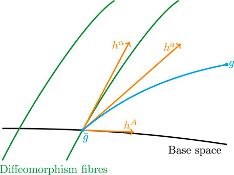
FIGURE 1. Illustration of the configuration space of metrics with the Vilkovisky connection. The background metric
The relation between g and
We close this section with some remarks on the implications of such a geometrical setup for “physical” gauge fixings, linear and exponential splits, and locality. The geometrical construction comes as close as possible to the definition of the configuration space of a gauge theory in terms of “physical” gauge-invariant fields and correlation functions. Such a parameterization is tantamount to a specific gauge fixing as already mentioned in Section 2.2. We may call such a gauge fixing “physical,” having in mind that it removes most of the redundancies related to the gauge group, in gravity that related to the diffeomorphism group. Note however that the terminology “physical gauge fixing” is not well-defined and also used differently in other contexts. In non-abelian gauge theories, the projection is unique and singles out the Landau–DeWitt gauge as the “physical” one. In gravity, one is left with a one-parameter family of gauges with the gauge fixing parameter β (see 7).
It is worth emphasizing that a gauge fixing condition for the geometrical field (or Gaußian normal field)
Finally, the geometrical construction with the Vilkovisky connection is highly nonlocal in configuration space, one of the ensuing problems being caustics and Gribov copies. This also raises the question of locality in the configuration space and that of momentum locality of the correlation functions of the geometrical fluctuation field h. The latter is discussed in detail in Section 7.4. Both locality issues highlight the challenges for manifest gauge- or diffeomorphism-invariant functional approaches to quantum gravity.
4 Flow Equation for Gravity
With the quantum field theory approach to quantum gravity outlined in the last sections, we are now in the position to discuss the flow equation approach to gravity. (For reviews, see 7–17, and for generic fRG reviews, see 18–27.) As already mentioned in the introduction of Section 3, the fRG approach to gravity is based on a successive integrating out of quantum fluctuations. Typically, this is done with an ordering of quantum fluctuations in momentum space: the regulator introduces a suppression of low-momentum fluctuations below an IR cutoff scale
Remarkably, the flow equation is insensitive to field reparameterizations of quantum gravity discussed in the last section or even physically different formulations: For the derivation, let us assume that a finite generating functional for correlation functions of the fluctuation field is given. In terms of a path integral, this is given by 13 with an assumed diffeomorphism-invariant regularization and renormalization procedure. More generally, such a finite generating functional is given by its defining property 14 under the assumption that these correlation functions are finite. Then, the flow equation can be readily derived without the necessity of referring to a specific representation of
The flow equation for the effective action is derived from the IR regularized generating functional,
with a
It is convenient to write the regulator
where momentum-squared is counted in cutoff units. In these units, the IR regime is given by
The first limit, 27a, guarantees the IR suppression of momentum modes. For example, for a scalar field in d dimensions with a quadratic dispersion
The second limit, 27b, guarantees that the UV behavior of the theory is unchanged by the IR regularization. We shall see below that the limit in 27b has to be approached sufficiently fast. In our example of a scalar field in d dimensions, the regulator shape function has to decay with at least
Subject to the existence of a finite full generating functional
where the RG-“time” t is defined with
The term in parenthesis in 28 is nothing but the full two-point correlation functions of the theory: the first term is the connected part, that is, the scale-dependent propagator
where
The flow equation for the effective action [2, 78, 79] follows straightforwardly from 28. The part proportional to
where
The flow equation for the effective action depends on the second derivative of the effective action with respect to the fluctuation fields,
for general functionals of
The different parameterizations of the metric field, discussed in Section 3, do not influence the flow equation for the effective action 31, and they only differ by their corresponding expansion schemes induced by the relations between metric and fluctuations (20, 21, 24). Still, from the viewpoint of diffeomorphism-invariance, the different parameterizations differ qualitatively. While the geometrical approach with the fluctuation field 24 by construction leads to a diffeomorphism-invariant effective action at all cutoff scales, diffeomorphism-invariance is broken in the linear split (20) and the exponential split 21 at a finite cutoff scale.
For all field parameterizations, a diffeomorphism-invariant effective action with one metric g is obtained at vanishing fluctuation graviton field
the background effective action. Its flow equation is given by 30, evaluated at vanishing fluctuation field
Importantly 34 is not closed: the right-hand side depends on
5 Background Field Approximation
The background field approximation, introduced in [3, 80] for YangMills theory and gravity, respectively, is the most commonly used approximation in the fRG approach to quantum gravity (see the reviews 7–16). It elevates the diffeomorphism-invariance of the background effective action to that of the full effective action. To that end, we write the full effective action in an expansion about the background effective action in 33,
The gauge fixing term
The underlying assumption is that the dynamics of a gauge theory is carried by gauge-invariant fluctuations, while
In the approximation 35 and with the linear split 20, the second derivatives of the effective action with respect to the background metric and the fluctuation field agree at
Inserting 35 into 30 leads us to a closed and diffeomorphism-invariant flow for the background effective action
5.1 Properties of the Background Approximation
It is the simple relation 36 and the manifest diffeomorphism-invariance of the approximation at all cutoff scales that make the background field approximation so attractive. A large amount of the results in asymptotically safe quantum gravity has been obtained in this approximation, and it is still the commonly used approximation in the field. This asks for independent checks of these results and its embedding in systematic expansion schemes that go beyond it. In the present work, we review the fluctuation approach (see Section 7), which includes the correlation functions of the fluctuation graviton field h. The results in the background field approximation are qualitatively in line with the results in the fluctuation approach discussed in Section 8. This confirms—in most cases—the underlying assumption 35b. Nonetheless, some words of caution are needed.
Despite its seeming manifest diffeomorphism-invariance, the background field approximation is at odds with diffeomorphism-invariance and background independence. To understand this counterintuitive remark, we recall some features of the background field formalism to standard quantum field theories, for example, the SM and QCD. The introduction of the background field to the gauge fixing allows defining a gauge-invariant background effective action. It is evident from its introduction that it is an auxiliary symmetry. The background field can even generate gauge-invariant background effective actions in theories that explicitly break gauge-invariance. This is clear from the construction of diffeomorphism-invariant background effective actions in gravity in the presence of a background-covariant momentum regulator. In a gauge-invariant theory without a cutoff, it can be shown that the physical gauge-invariance of the theory is carried by the fluctuation field in terms of nontrivial Ward– or Slavnov–Taylor identities. The underlying transformations are called quantum gauge/diffeomorphism transformations. This physical symmetry carries over to the auxiliary background gauge invariance via nontrivial Nielsen or split Ward identities. The latter encodes background independence of the theory and is introduced in Section 2.2. The Slavnov–Taylor and Nielsen identities for gravity are discussed in detail in Section 6.
In summary, only if the fluctuation correlation functions satisfy the nontrivial symmetry relations and the Nielsen identities, the auxiliary background gauge-invariance is physical. Then, it carries the underlying symmetry, and we have background independence.
5.2 Regulator Dependence of the Background Effective Action
In this section, we first argue that regulator choices within the general class defined with 26 and 27 can be used within the background field approximation to even change the (non-)existence or the nature of an asymptotically safe UV fixed point. This seems to casts some doubts on the reliability of results obtained in the background field approximation. However, we then show that the comparison with fluctuation results and the proper use of Nielsen identities (see Section 6) suffices to further restrict the general class of regulators such that it is adapted to the background field approximation.
The regulator term is the origin of the reliability problems of a naive use of the background field approximation within the fRG approach: it generates additional terms in
This has been discussed early on at the example of scalar theories and Yang–Mills theory in [81, 82]. In particular, it has been shown that the one-loop β-function in Yang–Mills theory can be changed from its universal result with regulator choices in the background field approximation. More precisely, it has been shown that for regulators,
(For details, refer to 82.) This spoils the universality of the one-loop β-function in the Yang–Mills theory. If one does not resort to the background field approximation, the correct one-loop β-function is obtained.
We now discuss the origin of this peculiar behavior. We follow the argument in [83] and for the general case including gravity (refer to [21, 72, 73, 83]). Simply put, we would like to show that the background effective action at a finite cutoff scale k and in particular in the limit
(see also 26). Note that in 38, we have introduced a
From the first term on the right-hand side of the flow 39, we deduce that the UV limit of the shape function is constrained:
This is a simple differential equation that admits a solution at least locally (in the flow time t). Note that the UV decay of
Equation 41 constrains the IR limit of the function
Apart from these trivial constraints, the choice of
The term
We emphasize that the result 42 is exact and no approximation has been applied. Equation 42 implies that without suitable restrictions on the regulator function
The IR limit with
does effectively not restrict the UV scaling. The latter is dominated by the UV-relevant operators that satisfy 43 by definition. Note that so far, we have discussed the flow of the background effective action
The above issues are already present for the full flow and emphasize the auxiliary nature of the background effective action at
Physical diffeomorphism-invariance and background independence are carried by nontrivial Slavnov–Taylor and Nielsen identities of the fluctuation field.
The background field dependence of the regulator term is potentially dangerous in the UV and has to be separated.
A first step in the resolution of the issues of the background field dependence is to monitor the field-dependence that originates in the regulator. The related equation and discussion in the Yang–Mills theory and gravity can be found in 21, 72, 73, 82, 83, 85, 86. (For applications to gravity, see also 57, 87–90.) The equation that monitors this dependence is given by
Equation 44 allows to disentangle the background-metric dependence stemming from the regulator from the rest. In the Yang–Mills example from 37, it can be shown that the regulator-field dependence is responsible for a contribution
Based on this analysis it has been suggested in 81, 82, that within the background field approximation, the corresponding field-dependence should be subtracted before applying the approximation
6 Symmetry Identities
Physical observables are diffeomorphism-invariant and background-independent. The underlying symmetry is dynamical and is solely carried by the dynamical fluctuation fields. It is called quantum diffeomorphism invariance and reads
The background metric triggers an a priori auxiliary symmetry, the background diffeomorphism invariance. It is given by the transformation
Here,
Both tranformations, 45 and 46, generated diffeomorphism transformations on the full metric
Any fRG computation needs to introduce a gauge fixing and a regularization, which both apparently break diffeomorphism invariance and (on-shell) background independence. Thus, it is an important issue in the fRG approach to quantum gravity to discuss how these properties can be preserved in a nonperturbative computation. For each symmetry broken by the cutoff term, we can formulate a nontrivial modified symmetry identity, which captures the cutoff deformation of the underlying symmetry and smoothly approaches the unbroken symmetry identity at vanishing cutoff scale,
6.1 Background Independence
As discussed in Section 2.1, we always need to split the full metric into a background metric
For example, in the linear split 20, we have
Let us first discuss the Nielsen identities without the regulator. The Ward identity for the effective action for any symmetry transformation
where
where
The Nielsen identity for the exponential split 21 resembles 51: there is a nontrivial difference between the background-metric and fluctuation-field derivatives due to the gauge fixing and ghost terms. In 17, we have pointed out that at
In comparison, for the fully diffeomorphism-invariant Vilkovisky–DeWitt or geometrical effective action with the split given by 22, the dependence on the gauge fixing action and the ghost action is vanishing, and thus, the Nielsen identity reads
In contradistinction to the linear and exponential split, the
The Nielsen identities entail that for all metric splits, the effective action is not a function of the full metric g but depends separately on the background metric
So far, the analysis has been performed in the absence of the cutoff term, that is, at
Note that in the last term in 53, only the metric fluctuation h contributes as the other fluctuation fields do not depend on the background metric. Furthermore, in the linear split, the last term is vanishing, and consequently, the mNI simplifies to
While some of the properties and consequences of the mNI are theory-dependent, most of them are generic, and much can be learned about applications in gravity from investigations in general theories: mNIs have been discussed in detail gravity, gauge theories, in scalar theories [3, 15, 21, 57, 72, 73, 81, 82, 87–93, 98–106].
There is an important qualitative difference between the breaking of the metric split symmetry 48 at finite k and at
(For a detailed discussion, see 97, 106, 107). The difference between the solutions can be parameterized by a term proportional to the regulator
The difference between
where V is the space-time volume and
which is displayed in the right panel of Figure 2 at the UV fixed point for different numbers of scalar fields
and thus, the quantum EoM is simply
This is shown in the left panel of Figure 2 at the UV fixed point for different numbers of scalar fields
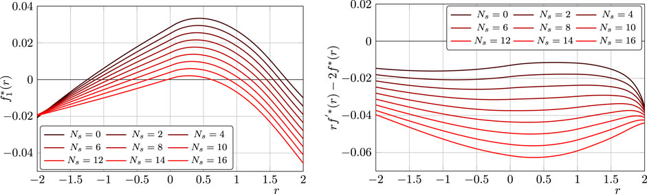
FIGURE 2. Displayed are the potential of the one-point function and the derivate of the background potential for different numbers of scalar fields at the fixed point, as defined in 57 and 59. A zero in these functions indicates a solution to the quantum and background EoM, respectively. While the former always has two solutions, a minimum at negative curvature and a maximum at positive curvature, the latter shows no solution at all. The figures are taken from 97.
The background EoM does not display a solution in the whole investigated region, while the quantum EoM has two solutions, a minimum at negative curvature and a maximum at positive curvature. For a larger number of scalar fields, these two solutions merge. However, in this regime, the approximation lacks reliability due to large values of the graviton anomalous dimension. Importantly, Figure 2 manifests in explicit computation the difference between the background and quantum EoM, 55. The background EoM was also extensively investigated in the background field approximation with different choices of regulator and parameterization. For example, in 108, the linear split was used and a solution at large negative curvature was found. However, in 109, 110, two further solutions at positive curvature were found due to a different choice of the regulator. A solution at positive curvature was also found in 111 and with the exponential parameterization in 51.
In 106, a modification of the fRG equation was proposed. There, the effective action was defined as the Legendre transform of a normalized Schwinger functional,
6.2 From BRST to Diffeomorphism Invariance
While the auxiliary background diffeomorphism invariance 46 remains unbroken, the physical quantum diffeomorphism invariance 45 turns into a BRST symmetry due to the gauge fixing, which is then further broken by the regulator. The related symmetry identities are called (modified) Slavnov–Taylor identities [(m)STI] [112, 113]. They encode physical diffeomorphism invariance. We sketch the main ideas of the derivation and apply them to gravity.
In case of the linear gauge fixing condition 7, the generator of BRST transformation (or BRST operator) denoted by
In (B), the vector field
For the derivation of the STI, we include a source term
where
The source term
With these properties, we obtain the STI for the Schwinger functional,
This identity can be re-expressed in terms of the effective action. (See 21 for details.) Here, we just state the result for the STI in the absence of the cutoff term,
This equation is known as the quantum-master equation. The BRST variation of the effective action is given by
Equation 64 encodes diffeomorphism invariance at
Some of the properties of the mSTI are theory-dependent, but most of them are generic: mSTIs in the presence and absence of background fields in gravity and gauge theories have been discussed in detail in [3, 15, 21, 22, 57, 72, 73, 81, 82, 87–93, 98–106, 114‒132].
In summary, we have three symmetries:
The auxiliary background diffeomorphism invariance 46, which remains unbroken.
The quantum diffeomorphism invariance 45, which describes physical diffeomorphism invariance. It is broken and encoded in the mSTI 65.
The split symmetry 48, which guarantees background independence. It is broken as well and encoded in the mNI 53.
The relations between background and fluctuation correlation functions are summarized in Figure 3. The relation between two fluctuation correlation functions can be expressed either with an mSTI or with a combination of mNI and background diffeomorphism invariance. However, it should be noted that in a truncated nonperturbative computation these two possibilities of relating fluctuation correlation function do not agree with each other. Nonetheless, it can be used to check the error of the truncation. (See Section 7.1 for more details.)
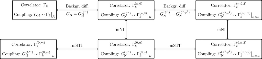
FIGURE 3. Displayed are the relations between background and fluctuation correlation functions in terms of symmetry identities. The background diffeomorphism symmetry 46 remains unbroken and trivially connects background correlation functions. The split symmetry (48) is encoded in the modified Nielsen identity (mNI) (53) and relates background correlation functions with fluctuation ones. The quantum diffeomorphism symmetry (45) is described by the modified Slavnov–Taylor identity (mSTI) 65 and relates fluctuation correlation functions. For the purpose of illustration, we have assumed that
Last but not least, the flow of mNI and the mSTI is proportional to itself, respectively. This is conveniently expressed in terms of the flow equation for composite operators, derived in [21, 128, 133]. Schematically, it reads
The operator
Equation 67 implies that once we have solved these identities at a scale k, then the identities are satisfied at all scales. However, this only holds for untruncated flows or truncations that are compatible with 67. (More details can be found in Section 7.1.)
6.3 Challenges for Diffeomorphism-Invariant Flows
Gauge-invariant approaches to quantum field theories have received much attention over the decades both in perturbation theory and beyond. Such formulations also have met considerable challenges, except for lattice gauge theories that are based on link variables formulated in the gauge group. In turn, perturbation theory and nonperturbative functional approaches are based on correlation functions and in particular on the propagator of the algebra-valued gauge field. (For reviews on lattice approaches to quantum gravity see, e.g., 140–144).
Gauge-invariant functional formulations are based either on gauge-invariant or gauge-covariant variables such as the geometrical formulation, the field strength formulation, or Wilson line formulations similar to lattice gauge theories. Implementations in the flow equation approach range from generalized Polchinski equations with gauge-covariant kernels for the Wilson effective action [145–156] and its recent manifestations [157–159], over the geometrical or Vilkovisky–DeWitt flows for the effective action [21, 71–74], to a recent suggestion for a gauge-invariant flow for the effective action [160–164].
Most of these approaches rely explicitly or implicitly on the definition of projection operators on the subspace of the dynamical degrees of freedom. Typically, this is achieved by a gauge fixing, but the notation of a projection is far more versatile. The appropriate definition of this projection and the respective geometrical structure of the configuration space is at the root of the geometrical construction. This has been discussed in Sections 3.3, 6.2, and 6.3, and we refer to the discussions there. The notable nonlocality of the projections both in field space as well as momentum space is an inherent property of the construction of gauge-invariant subspaces. Consequently, it should be considered an inherent feature of such a construction. This inherent nonlocality may be buried in functional self-consistency relations, but it is present explicitly or implicitly without any doubt.
In any case, the situation calls for self-consistency checks of the final formulations of gauge-invariant or diffeomorphism-invariant flows. This necessity has been discussed already in 165: there the terminology of complete and consistent flows was introduced. The former flows generate all quantum fluctuations from a given classical action, while the latter flows generate a well-defined subset of quantum fluctuations from a given—partial—effective action. A well-known example for the latter is thermal flows, which only generate thermal fluctuations from the full quantum effective action at vanishing temperature. In 165, 166, an important and simple consistency check for flow equations has been suggested: any complete flow equation must generate the complete perturbation theory upon iteration from the given classical action. While one-loop perturbation theory in the fluctuation field is trivially achieved within one-loop exact flow equations, two-loop perturbation theory provides a nontrivial necessary, while not sufficient, consistency check.
These checks for diffeomorphism-invariant fRG approaches have been passed for the Wilsonian approach [145–156] or are trivial for the geometrical effective action approach [21, 71–74]. It is a highly relevant and interesting question how the more recent proposals [158–164] fare in such a self-consistency check. Respective investigations either confirm the completeness of the approaches or may show their consistency, that is, they may integrate out a well-defined subset of quantum fluctuations. Finally, for potentially consistent flows, such an investigation may enable the construction of nontrivial two-loop consistent extensions. We emphasize that such an extension does not simply pass a two-loop test but more importantly allows for two-loop resummed nonperturbative approximations. The latter set of approximations certainly live up to the self-consistency of other state-of-the-art computations in asymptotically safe quantum gravity, while having the benefit of inherent diffeomorphism invariance.
7 Fluctuation Approach
In the last sections, we have detailed the need for an fRG approach to quantum gravity that goes beyond the background field approximation and that allows satisfying the nontrivial symmetry identities, the mSTI 65 and the mNI 53. For general metrics
This suggests the expansion of the effective action
Evidently, if the expansion coefficients
7.1 Hierarchy of Flow Equations
The background field approach leads to an extended hierarchy of flow equations. We first note that the background flow equation
In other words, we need
Equation 70 is the full hierarchy of integrated flow equations to solve for quantum gravity. While its solution in terms of the vertex expansion has been baptized the fluctuation approach, it simply is the full problem at hand.
Apparently, 70 constitutes a system of equations for a two-field effective action. However, as discussed in Section 6, background independence at vanishing cutoff,
This leaves us with two towers of functional relations. While the first one (70) describes the full set of correlation functions, the second one (71) can be used to iteratively solve the tower of mixed fluctuation background correlations on the basis of the fluctuating correlation functions
An important feature of the fRG equations is that in the Landau limit of the gauge parameter
In other words, the flow equation system of transverse fluctuation correlation functions is closed and determines the dynamics of the system. In the fluctuation approach, the transverse system of graviton correlation function has been solved up to the four-graviton vertex [184]. A diagrammatic depiction of the system of flow equations is given in Figure 4, and a description of the respective results can be found in Section 8.
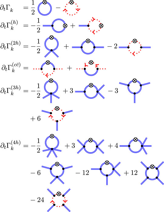
FIGURE 4. Diagrammatic representation of the flow equations of the fluctuation n-point functions up to
In turn, the flow equation system for longitudinal fluctuation correlation functions is not closed, and the transverse correlation functions
Note that
(See 185 for non-abelian gauge theories.) In consequence, the mSTIs provide no direct information about the transverse correlation functions without further constraint. In the perturbative regime at large momenta, this additional constraint is given by the uniformity of the vertices. In turn, in strongly correlated regimes such a general constraint is absent. Indeed, one can show that the confinement property in a Yang–Mills theory in a covariant gauge necessitates the absence of uniformity of the vertices at low momenta. (For a detailed discussion in non-abelian gauge theories, see 168.)
Instead, we can simply use 74 for a given set of transverse correlation functions for constructing a BRST-invariant solution, which signals diffeomorphism invariance. For a given finite set of transverse correlation functions, generically such a solution can be found by integrating the flow (67). However, it may be nonlocal. The existence of BRST-invariant solutions for a general transverse input emphasizes the fact that the derivation of diffeomorphism-consistent solutions is not necessarily the hallmark of a good truncation. However, the comparison of 74 and 73 is a further nontrivial constraint on longitudinal correlation functions. Its evaluation is complicated by the fact that the solutions of two different functional relations for the same set of correlation functions do not agree in general in nontrivial truncations. Furthermore, it is very difficult to provide a measure for the closeness of the solutions. (For a related discussion in non-abelian gauge theories, see the recent review [27] and references therein.)
In summary, the evaluation of diffeomorphism invariance and self-consistency constitutes an intricate challenge. One has to utilize all the properties and relations discussed above. This holds for all fRG approaches to quantum gravity and not only to the fluctuation approach: only local BRST-invariant solutions should be considered physical, and the evaluation of locality and BRST invariance or their absence is intricate.
7.2 Flat Expansion Is a Curvature Expansion
As briefly mentioned in the introduction of this section, the choice of the background metric is important for the convergence of the vertex expansion. However, an evaluation of the flow equations for
the Euclidean analog of the Minkowski metric. This has been baptized the flat expansion. With the flat background (75), Fourier transformations can be performed, and we are led to correlation functions
This expansion encompasses the standard curvature expansion with the additional benefit that generic covariant momentum dependences are systematically accessible. (For a respective brief discussion, see 184.) To understand this statement, we sketch the curvature expansion of the background field approximation with standard heat kernel techniques and the flat expansion in momentum space. We shall see that both lead to the same flow equations for the expansion coefficients of diffeomorphism-invariant operators. We expand the full one-field effective action in local curvature invariants and covariant derivatives
In 76, the first term on the right-hand side is the Einstein–Hilbert action with a scale-dependent cosmological constant and Newton coupling. The second term includes all other curvature invariants starting with
Similarly to 76, the flow of the background effective action can also be expanded in terms of local curvature invariants and covariant derivatives. This leads us to
with expansion coefficients
Evidently, any complete projection procedure produces the complete set of flow equations of all expansion coefficients
The standard procedure for projecting onto the flow of the cosmological constant and the Newton coupling, as well as that of higher order invariants, is by heat kernel techniques or explicit summation over the spectrum of the covariant Laplacians, in conjunction with the Euler–Maclaurin formula (see the reviews [7–16]). As no other local diffeomorphism-invariant operators are present at this order, the flow of
Now, we derive the flows in 78 within the flat expansion scheme. To that end, we note that the only local diffeomorphism-invariant term with no derivatives is the volume term
where the subscript TT refers to the projection and normalization on the traceless-transverse part. (More details can be found, e.g., in 184.) Equation 79 simply is 78, as the flat expansion scheme is a consistent projection scheme.
This procedure can be extended beyond the set of local diffeomorphism-invariant operators:
Take general derivatives with respect to
Contract with all possible Lorentz tensor structures.
Take derivatives with respect to momenta.
In particular, apart from all local diffeomorphism-invariant term, the expansion captures general covariant momentum dependences including potential IR-singular terms and topological terms. A diffeomorphism-invariant example for the former is the Polyakov action in two dimensions,
(see, e.g., 190, 191). IR-singular terms are naturally covered by taking into account full momentum dependences of full vertices or momentum channels of specific tensor structures. This has been used extensively in gauge theories such as QCD not only within the fRG approach but also in other functional approaches based on Dyson–Schwinger equations or n-particle irreducible hierarchies.
A relevant example for a topological term in gravity is the Gauß–Bonnet term with the density
Metric variations of the local density
Below, we outline a cautious approach guided by the works 192, 193 in gauge theories. There, a simple example for a topological invariant is the Pontryagin index in a
The auxiliary field
The tensor structure
where we have defined
The (local) total derivative property of the Gauß–Bonnet density is reflected in the fact that all
In summary, the flat expansion allows projecting the flow equation on the flow of all coefficients
Here,
The findings of the present section can be summarized as follows:
The flat expansion encompassed the curvature expansion. There is no conceptual difference, and both expansions are expansions about the flat background
The expansion point of the curvature or flat expansion is not the solution of the EoM,
The fluctuation approach within the flat vertex expansion resolves the difference between fluctuation and background field. As such it simply improves upon the background field approximation within the curvature expansion without introducing other approximations: fluctuation approach results benchmark that in the background field approximation and provide nontrivial reliability checks for the latter.
There are an increasing number of computations that do not rely on the curvature expansion, for example, 49, 51, 54, 109–111, 175–182 in the background field approximation and 97, 107 in the fluctuation approach. This concludes our discussion of the formal properties of the fluctuation approach.
7.3 Tensor Structure and Momentum Dependence of Vertices
In the flat expansion, the vertices
where,
which describes the running of the rescaled fields
where the sum over j is implied. The size of the complete set of tensor structures increases rapidly for higher order vertices. The cutoff-dependent dressings
In most applications to gravity, only the Einstein–Hilbert tensor structures deduced from the curvature scalar and the volume term are taken into account. This leads us to
with the Einstein–Hilbert action 1 and the momentum-dependent global dressing
For
7.4 Momentum Locality
An important property of a physical coarse-graining procedure is momentum locality: it ensures that a coarse-graining step at a given cutoff scale k does not influence the physics at momentum scales
In this definition, all momenta
The condition 91 is satisfied by all perturbatively renormalizable local quantum field theories of scalars, fermions, and vector fields (including gauge fields in linear gauges with linear momentum dependences) by trivial counting of the momenta. In turn, nonrenormalizable theories with nontrivial momentum dependences of vertices are easily nonlocal. For example, the scalar field theory with an interaction term of the type
Thus, a naïve momentum counting in gravity leads to the conclusion that the coarse graining is not momentum local, neither in Einstein–Hilbert gravity nor in a higher derivative theory of gravity. One needs nontrivial cancellations between diagrams. In 198, such a cancellation was observed for the first time in the transverse traceless part of the graviton two-point function with Einstein–Hilbert vertices. In 197, this was extended to the transverse traceless part of the graviton three-point function. Both cases are displayed in Figure 5. There are three diagrams (plus one ghost diagram) contributing to the flow of the graviton three-point function (Figure 4). The cancellation takes places between all diagrams and holds for all gauge fixing parameters and all momentum configurations of the three-point function, as long as all external and internal momenta are sent to infinity.
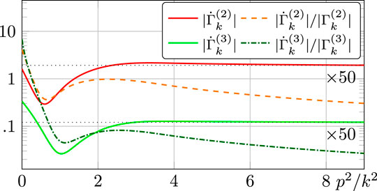
FIGURE 5. Displayed are the flows of the traceless transverse parts of the graviton two- and three-point functions,
We close this section with the remark that the results in 197, while highly nontrivial, should be considered to be the first step in a fully conclusive analysis. Most notably, the observed locality does not hold for all tensor structures of the n-point functions considered there. In our opinion, this may hint at persistent nonlocalities introduced by the gauge fixing. If this can be solidified in further investigations, this should allow for selecting gauge fixings that make the coarse graining procedure for a given regularization procedure momentum local. Note that while momentum locality of a coarse graining procedure is not a necessary property, it certainly improves the convergence of standard approximation schemes which are typically momentum local. Moreover, if no momentum local coarse graining procedure can be found for a given theory, this casts serious doubts on the interpretation of such a theory as a local quantum field theory.
8 State of the Art
We are now ready to review the state of the art of asymptotically safe quantum gravity within the fluctuation approach. To facilitate accessing the relevance of the different results for the self-consistency of the approach, we start with a brief overview:
UV Fixed Point (Section 8.1): The existence of a UV fixed point with a finite-dimensional critical hypersurface ensures the UV finiteness and predictivity of the theory. With the fluctuation approach, this has been investigated for pure gravity in 73, 93, 97, 107, 184, 197–206. The UV fixed point is comparable with results in the background field approximation and thus consolidates these results. Three UV-attractive directions are found associated with
UV-IR Trajectory (Section 8.2): A UV-IR trajectory allows us to connect to a classical GR regime and IR-SM physics if matter couplings are included. Classical GR regimes are accessed for
Momentum Dependence and Unitarity (Section 8.3): The full momentum dependence, in particular of the propagator, opens a path toward a first investigation of unitarity via spectral reconstructions. The truncations already include the momentum dependence of the graviton two-, three-, and four-point functions at the momentum symmetric point [184, 197, 198] as well as the momentum dependence of the graviton-matter three-point vertices [93, 202–204]. The momentum dependence has been also used to show the absence of IR divergences in the IR regime [198, 199] and to show the absence of
Curvature Dependence (Section 8.4): The curvature dependence of the correlation functions allows extending the results from a flat background to a generic background. The full curvature dependence of the fluctuation correlation functions contains the information of the diffeomorphism-invariant effective action (Section 7.1). The first steps in this direction in pure gravity and scalar gravity systems have been done in 97, 107, 206. In 97, 107, the difference of the background and quantum EoM due to the mNI was explicitly computed (see Section 6.1 and Figure 2).
Gravity–Matter Systems (Section 8.5): The aim is to incorporate the SM degrees of freedom in asymptotically safe quantum gravity and eventually to retrodict SM parameters and to constrain beyond the SM physics [207–218]. Minimally and nonminimally coupled gravity–matter systems have been investigated with (partial) fluctuation approach techniques in 53, 83, 93, 97, 187, 202, 204, 219–224. A particularly interesting question is for which matter content the UV fixed point exists. First bounds were computed in 219; however, a qualitative difference between the results in the background field approximation and the fluctuation approach was found [220]. It was shown in 202 that higher order curvature terms are needed to fully address this question. (For gravity–matter systems with higher derivative gravity in the background field approximation, see 58, 183, 186.) The investigation in 97 is a first step toward the computational confirmation of the existence of an asymptotically safe fixed point for general gravity matter in the minimally coupled approximation. This opens a path toward reliable stability investigations of fully coupled gravity–matter systems.
Effective Universality (Section 8.6): Last, we discuss the potential close perturbativeness of the UV fixed-point regime of asymptotically safe gravity. This leads us to the concept of effective universality: the so-called avatars of the Newton coupling extracted from different correlation functions may agree up to differences that can be inferred from the modified STIs that relate these couplings [93, 203]. If present, effective universality may have a dynamical origin. The analysis of this intriguing property is also intricate due to truncation artifacts and RG scheme dependences. We close this overview by commenting on the related bimetric approach and hybrids of the background field approximation and the fluctuation approach.
Hybrid approaches: In hybrid approaches, one substitutes part of the fluctuation flow equations with background flow equations [66, 219, 225–232]. In most cases, this concerns the notoriously difficult pure gravity couplings: the derivation of fluctuation flows of pure gravity vertices such as the three- and four-point functions requires a significant computer algebraic effort. In advanced truncations, this is accompanied with numerical loop integrations in every flow step and interpolations of dressing functions with potentially several momentum and angular dependences. In turn, using the background field approximation for these vertices reduces this task to computing the flow of a single background coupling, whose flow equation is known analytically. This considerable reduction makes it chiefly important to construct reliable background field approximation schemes as discussed in Section 5.2
An alternative to the use of the background field approximation for the pure gravity couplings is their identification with matter–gravity couplings. Such an identification implicitly relies on the concept of effective universality discussed in more detail in Section 8.6. There it is discussed that while the full system shows effective universality, it is only maintained if using the pure gravity couplings for the matter–gravity couplings. In turn, effective universality, as well as the compatibility with the full system, is lost if using the matter–gravity couplings as pure gravity ones. This hints at a surprisingly complicated interaction structure in gravity–matter systems whose origin is yet to be understood.
Bimetric approach: The bimetric approach, developed in 100–102, 233, is tantamount to the fluctuation approach reviewed here, as it rests on the distinction between the background metric and the fluctuation field. Technically, fluctuation and background correlation functions are defined in terms of an expansion of the full metric
in analogy to 68. The
8.1 Ultraviolet Fixed Point
The UV fixed point in the fluctuation approach has been discussed in 73, 93, 97, 107, 184, 197–206. This includes work in the vertex expansion about the flat background in pure gravity [184, 197–200] and gravity–matter systems [93, 201–204] as well as work including curvature dependence [97, 107, 206], a fluctuation potential [205] and in the geometrical approach [73]. In 184, the tower of fluctuation correlation functions was implemented until the graviton four-point function. All n-point functions were evaluated at the momentum-symmetric point, with external transverse traceless projections. A UV fixed point was found at
where
where a positive sign corresponds to a UV-attractive direction. The three UV-attractive directions were associated with the operators
In Section 7.2, we have shown that the fluctuation approach in the flat expansion improves upon the background field approximation in the curvature expansion (see in particular the discussion at the summary at the end of Section 7.2). Accordingly, the fluctuation results for the UV fixed point detailed above extend and corroborate previous findings in the background field approximation within the curvature expansion. In particular, the results confirm that the latter captures the most important features in pure gravity. For example, the fixed-point value of the cosmological constant in the background field approximation is typically positive, which is comparable with the negative fixed-point value of µ in 93 (
A further extension, within the exponential split, has been investigated in 205. There, the dimensionless fluctuation potential V was approximated with
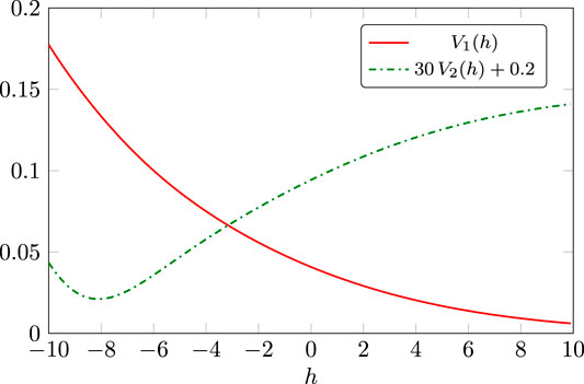
FIGURE 6. Dimensionless fixed-point fluctuation potentials defined via
8.2 Ultraviolet–Infrared Trajectories
UV-IR trajectories in the fluctuation approach and hence the phase structure of quantum gravity have been discussed in 73, 184, 198, 199. In Figure 7, we display a trajectory from the UV fixed point (93) to the IR where all couplings run classically. In the displayed example, the graviton mass parameter runs to infinity,
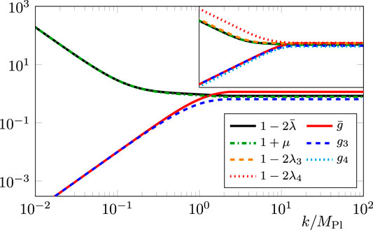
FIGURE 7. Scale dependence of different fluctuation couplings along a trajectory from the UV fixed point 93 to the IR. In the IR, the couplings flow according to their canonical running. For small k,
Moreover, the background Newton coupling and (all) the fluctuation Newton coupling agree. This can be seen for the dimensionless versions
UV-IR trajectories with
8.3 Momentum Dependence and Unitarity
The momentum dependence of correlation functions have been discussed in 93, 184, 197–199, 202–204. This momentum dependence encodes the dynamics of the theory and is crucial for the question of unitarity. One of the advantages of the fluctuation approach in the flat vertex expansion is its easy access to the full momentum dependence of fluctuation correlation functions
at vanishing fluctuation field
Equation 96 entails in particular that any observable inherits its dynamics from that of the full field and momentum dependence of the fluctuation two-point function, or rather from the momentum dependence of the fluctuation correlation functions
Moreover, the resolution of the momentum dependences of n-point functions gives at least indirect access to the question of unitarity of asymptotically safe gravity: From the Euclidean data, one can reconstruct Minkowski correlation functions and in particular the graviton spectral functions, both that of the fluctuation graviton and that of the background graviton (more details will be given in 235). Here, we simply comment on the physics content of the graviton spectral functions (see also 236). In this context, we will also use the analogy to the gluon in a non-abelian gauge theory as discussed in 237. (For a recent discussion of the challenges for unitarity in asymptotically safe gravity, see 16.)
To begin with, both the fluctuation graviton and the background graviton two-point functions are not diffeomorphism-invariant. Accordingly, they are not directly related to asymptotic states; even at low energies, gravity is weakly coupled and the theory exhibits a classical momentum and scale dependence (see Figure 7). The latter property suggests that if a Källén–Lehmann spectral representation of the graviton propagators exists, the graviton spectral functions may exhibit a particle-like spectrum for low spectral values. In turn, for large spectral values, we enter the UV fixed point regime, and the physics content of the spectral functions is unclear.
Note however that the same line of arguments would suggest that the gluon spectral function exhibits a particle-type spectral dependence in its perturbative regime for large spectral values. Instead, it can be shown that if a Källén–Lehmann spectral representation exists, the gluon spectral function is negative for large spectral values, and its spectral sum vanishes (Oehme–Zimmermann superconvergence relation). Moreover, it is also negative for small spectral values (see 237). These properties hold for both the fluctuation and the background gluon. Since these properties follow directly from the momentum dependence of the Euclidean correlation functions, we expect similar results for asymptotically safe gravity [235].
In summary, the spectral properties of diffeomorphism- or gauge-variant correlation functions only indirectly mirror the unitarity of the theory. This situation prohibits any direct conclusion of a lack of unitarity from the occurrence of negative parts of spectral functions including negative poles (ghost states). We also emphasize that the latter statement should not be taken as its converse. Of course, the occurrence of negative parts of spectral function requires a thorough investigation of the physics implications and may well be related to the lack of unitarity of the underlying theory. The example of the non-abelian theory simply indicates that this is not necessarily the case. Such an investigation requires the analysis of the spectral properties of diffeomorphism-invariant states. (For a recent discussion of such a setup, see 196.)
The discussion in this section so far emphasizes the importance of the computation of the momentum dependence of correlation functions both for the dynamics of observables and the intricate problem of unitarity. One of the advantages of the fluctuation approach is the direct access to momentum-dependent correlation functions with standard quantum field theory methods:
In 198, 199, the full momentum dependence of the graviton and ghost propagator was included via the anomalous dimensions. The computation of the momentum dependence was extended to the graviton three- [197] and four-point function [184] as well as to the scalar–graviton [93], the fermion–graviton [204], the gluon–graviton vertex [202], and the ghost–graviton vertex [203]. While only the momenta
In 184, 200, the momentum dependence was used to disentangle contributions from the couplings of the
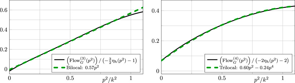
FIGURE 8. Momentum dependence of the transverse traceless graviton three- and four-point couplings obtained by normalizing the vertex flow with
Recently, impressive progress has been made toward momentum-dependent computations in the background field approximation [238–242]. There, the momentum dependence is captured via form factors
8.4 Curvature Dependence
The curvature dependence of correlation functions in the fluctuation approach has been discussed in 97, 107, 206. Most results in the fluctuation approach were computed on a flat background
A different approach within the fluctuation approach was taken in 97, 107, where the fluctuation correlation functions were computed directly on a generic background with constant curvature. The computation reaches up to the graviton three-point function and also includes
8.5 Gravity–Matter Systems
A theory of quantum gravity necessarily needs to include matter degrees of freedom to describe our universe. A central question is for which matter content, the UV fixed point exists and if certain types of matter field have a stabilizing or destabilizing effect. Most studies have focused on analyzing SM matter fields within the minimally coupled approximation. In this approximation, the matter fields are considered without self-interaction and only couple to gravity via their kinetic term. There are works in the background field approximation [58, 183, 186, 243–249], in the hybrid approach [53, 219], and in a full fluctuation computation [93, 97, 201–204]. (For works beyond the minimally coupled approximation, see 47, 50, 83, 162, 186, 188, 210, 220–224, 228, 229, 232, 250–260, which also includes scalar–tensor theories and gravitational corrections to the running of matter couplings.)
A major keystone in the stability analysis of gravity–matter systems in the minimally coupled approximation was found in 201, 202. There, it was shown that minimally coupled gravity–matter systems in the Einstein–Hilbert truncation always show a Reuter fixed point as the system can be mapped to a pure gravity system at the level of the path integral. We emphasize that while the explicit computations in 201, 202 are done in the fluctuation approach, the conceptual investigation is general. (For a detailed discussion we refer to 202.) Here, we simply sketch the important steps: In minimally coupled gravity–matter systems, the matter part
with
Here, the full fluctuation field is split into
The form of the generating functional in 97 is also obtained for UV-complete non minimally coupled matter theories such as Yang–Mills theories. Then,
The representation 97 emphasizes an intriguing and useful property of the fRG approach to quantum gravity (and beyond): The phase structure and in particular the fixed-point structure of a generic gravity–matter system can be accessed within pure gravity. In particular, all fixed points are accessible within this setup, if a general fixed point effective action
This intriguing property also carries an important intricacy of a generic fixed-point analysis: Seemingly, the parameterization 97 entails that generic gravity–matter systems are UV-stable if the matter part is UV-complete (with the assumption that the Reuter fixed point exists for pure gravity). This conclusion would apply directly to all minimally coupled gravity–matter systems. That this argument falls short can be seen at the example of many-flavor QCD. There, an (f)RG analysis reveals that the QCD β-function changes its sign for a large enough number of flavors. In the vicinity of this regime, interesting phenomena such as conformal scaling, instabilities, and the Caswell–Banks–Zaks fixed point occur (For fRG literature, see, e.g., 261–264 and references therein.) These findings are backed up by lattice results. The RG analysis in many-flavor QCD solely relies on the marginal operator
where
and similar ones for
The logarithmic RG running of the marginal operator
In summary, from the perspective of the Yang–Mills system with the generating functional similar to that in 98, the marginal operator 99 introduces a new UV marginal (and hence physical) parameter
The above properties imply that a fixed-point analysis of a given system within a truncation of the (f)RG flows that does not include the flows of the marginal operators should exhibit the respective fixed-point structure of the pure gravity system in the same truncation. In particular, this casts some doubt on any instability findings in the full truncation, if this instability survives in the absence of the marginal operators.
As an example of this statement, we consider now a minimally coupled gravity–matter system in the Einstein–Hilbert truncation. Without truncation, these systems have the path integral representation 97 with 98. The Einstein–Hilbert truncation reduces
where the subscript
The above result for minimally coupled systems has the direct consequence that the Einstein–Hilbert truncation to matter–gravity systems should also exhibit the Reuter fixed point for UV-complete matter systems, as the pure gravity system does. We add that this does not exclude the emergence of further fixed points in some
This concludes our discussion of the fixed-point structure and stability properties of gravity–matter systems, its truncation dependence, and reliability requirements for truncations. The discussion enables us to formulate relevant properties that have to be considered for a conclusive stability analysis of matter–gravity systems:
The fixed-point analysis necessarily has to involve all (possibly) relevant operators of the theory under investigation, that is, 99 in many-flavor QCD and 100 in gravity–matter systems.
A fixed-point analysis within a given truncation is only fully reliable if it also reproduces the fixed-points of the pure gravity system in the same truncation excluding the marginal operators.
We now discuss the results in gravity–matter systems given the properties i) and ii): In [201], the first full fluctuation computation for minimally-coupled systems was put forward. On the pure gravity side, the flows of the fluctuation graviton two- and three-point function were included. Importantly, a stabilizing mechanism for the fermionic contribution was found for general regulators: the graviton mass parameter is approaching its pole
In the same truncation applied to minimally coupled scalar–gravity systems, it was found within the fluctuation approach in 93, 201 that the graviton anomalous dimension
Applying the same truncation to minimally coupled gauge–gravity systems, it has been shown in 202 that depending on the regulator, the minimally coupled systems either behave similarly to the fermionic or the scalar system. This suggests that the truncation has to be improved. In summary, a stability analysis of gauge–gravity systems can be performed, but the results have to be taken with a grain of salt. A fully conclusive stability analysis for gauge–gravity systems requires an improvement of the truncations used so far in the literature.
In Figure 9, we display the state-of-the-art dependence of the fixed-point values on the number of scalar field
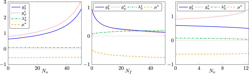
FIGURE 9. Fixed-point values of the fluctuation couplings as a function of the number of scalar (left), fermion (middle), and gauge fields (right). All truncations include the graviton two- and three-point function as well as the respective graviton–matter vertex. In the scalar case, the Newton couplings,
Finally, we speculate on the stability properties of general gravity–matter systems based on the results obtained so far. To that end, we assume that there is a setup such that general minimally coupled gravity–matter systems in the Einstein–Hilbert truncation show UV stability with a Reuter fixed point similar to the one seen in the fermion–gravity system. This property allows for a consistent truncation as it satisfies ii). Now, we include tensor structures from curvature-squared terms,
with the dimensionless couplings
We concentrate on the Reuter fixed point with the assumption that it is dominated by the Einstein–Hilbert couplings in contradistinction to the perturbative
Moreover, from the quartic term
Switching off the Einstein–Hilbert contribution leads us to the standard Gaußian fixed point for
in pure gravity. We add that the relevance analysis in 184 suggests that the
We now proceed to the
The right-hand side has a form similar to the flow equation itself and is UV- and IR-finite. Accordingly,
where we have used that the dimensionless coefficient
The above considerations allow us to discuss the generic structure of gravity matter flows within the fluctuation approach,
where
The quantitative evaluation of 108 depends on the full fluctuation flows in pure gravity including flow contributions from curvature-squared invariants. Here, we concentrate on the structure of the β-function of the
We close this chapter with a brief overview of investigations of gravity–matter systems within the background field or hybrid approximations. In 219, gravity–matter systems in the minimally coupled approximation were investigated in a hybrid approach: while most contributions to the flow have been computed in the background field approximation, the matter parts of the anomalous dimensions have been computed in a fluctuation approach setup. Within this approximation, destabilizing effects for scalars and fermions and stabilizing effects for gauge fields were found. The destabilizing result for fermions in 219 is an artifact of the background field approximation, as discussed in destabilizing result for Section 8.5: the background-metric dependence of the regulator influences the (de)stabilizing property of minimally coupled fermions. However, this does not imply that the background field approximation breaks down for all gravity couplings. The results of 201, 202 showed that in particular, the most UV-relevant operators have to be taken from a fluctuation computation, that is, most importantly the graviton mass parameter µ. In turn, the background and the fluctuation Newton coupling behave rather similar under the influence of minimally coupled matter fields. The sign of leading-order contribution agrees: the scalar and fermionic contribution to the beta function of the Newton coupling at
In summary, the investigations of gravity–matter systems within the fluctuation approach open a systematic path toward reliable stability investigations of fully coupled matter systems as well as that of phenomenological consequences for high energy physics. Still, fully reliable results require a systematic and qualitative improvement of the current truncations. This is the subject of current work in the community.
8.6 Effective Universality
In the vertex expansion 68, we have introduced the couplings
This is similar in non-abelian gauge theories, where different avatars of the running strong coupling
In gravity, the situation is even more intricate. To begin with, the Newton coupling is dimensionful, and hence, the β-functions of the avatars of the Newton coupling are not universal, leaving aside an identical momentum dependence. Additionally, as already mentioned in the context of non-abelian gauge theories, the standard fRG renormalization schemes are typically mass-dependent, which adds to the differences, as do truncations.
Effective universality is the concept that in particular at the fixed point, where gravity is in a scaling regime, and the quantum theory is dominated by the diffeomorphism invariance of the underlying theory. If this scenario applies, the β-functions and the momentum dependence of different avatars of the Newton coupling should agree or are rather be close to each other on the asymptotically safe UV fixed point. This concept would apply to all couplings, and in particular, the
Given the presence of truncations in explicit computations, the impact of nontrivial mSTIs and the nonperturbative nature of the UV fixed point, it is left to define a measure for effective universality. In 93, 203, it was quantified how these avatars differ at the UV fixed point using the measure
where
In 203, five avatars of the Newton coupling were included stemming from the three-point functions,
The universality measures
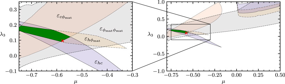
FIGURE 10. Effective universality of the different avatars of the Newton coupling as a function of µ and
We emphasize that the observed effective universality is a highly nontrivial result. If it can be sustained in further analyses, it is presumably dynamical. This conjecture is supported by the following observation: for a marginal universal coupling, one may simply compute one avatar of the coupling and identify the other avatars with the computed one. In turn, in a theory like gravity, where the effective universality is potentially generated dynamically, this may only work in specific RG schemes. One may even define a natural RG scheme by
In any case, within a given RG scheme, some of the β-functions may satisfy
In gravity–matter systems, we indeed observe, in given truncations, such a behavior: if all avatars of the Newton coupling are identified with the three-graviton coupling
9 Summary and Outlook
In this contribution, we have reviewed the state of the art of the fluctuation approach to quantum gravity. This approach is based upon the computation of the correlation functions of the dynamical graviton fluctuation field
By now, the fluctuation approach has matured (see the overview of the results in Section 8). We see signs of apparent convergence of the results in pure gravity. Moreover, by now, we can reliably evaluate the stability of general gravity–matter systems. In combination, the fluctuation approach now allows for reliable physics predictions for the UV regime of asymptotically safe gravity including its unitarity. The approach also allows for reliable physics predictions for the “IR” particle physics within the asymptotically safe standard model.
Author Contributions
All authors listed have made a substantial, direct, and intellectual contribution to the work and approved it for publication.
Funding
This work is supported by the DFG, Project-ID 273811115, SFB 1225 (ISOQUANT), as well as by the DFG under Germany’s Excellence Strategy EXC - 2181/1–390900948 (the Heidelberg Excellence Cluster STRUCTURES), by the Danish National Research Foundation under Grant No. DNRF:90, and by the Science and Technology Research Council (STFC) under the Consolidated Grant ST/T00102X/1.
Conflict of Interest
The authors declare that the research was conducted in the absence of any commercial or financial relationships that could be constructed as a potential conflict of interest.
Acknowledgments
We thank A. Bonanno, B. Bürger, N. Christiansen, T. Denz, A. Eichhorn, K. Falls, H. Gies, A. Held, B. Knorr, P. Labus, S. Lippoldt, J. Meibohm, D. Litim, A. Pereira, A. Rodigast, B.-J. Schaefer, M. Schiffer, F. Saueressig, J. Smirnov, M. Yamada, and C. Wetterich for discussions and work on the subjects reported on.
Appendix a notation
Our convention for functional derivatives are given by
where the parenthesis in the superscript of the Kronecker-δ’s stands for the symmetrisation of the indices including a normalisation factor
This leads to the correlation functions of the fluctuation fields as given in Ref. 14.
The metric
with the Northwest-Southeast convention
These definitions entail
more details can be found in Ref. 21.
Appendix b pontryagin index in u(1) gauge theories
The Pontryagin index P of a four-dimensional
with the Pontryagin index
In momentum space
The flow of θ has been studied in Ref. 193 for the topological charge in Yang-Mills theories. Two derivatives with respect to the gauge field in momentum space lead us from Eq. B8 to
For a topological term with constant
References
1. Weinberg S. General relativity: an Einstein centenary survey. SW Hawking, and W Israel editors. Cambridge, England: Cambridge University Press (1980)
2. Wetterich C. Exact evolution equation for the effective potential. Phys Lett B (1993) 301 (1):90–4. doi:10.1016/0370-2693(93)90726-x
3. Reuter M. Nonperturbative evolution equation for quantum gravity. Phys Rev D (1998) 57:971–85. doi:10.1103/physrevd.57.971
4. Souma W. Non-trivial ultraviolet fixed point in quantum gravity. Prog Theor Phys (1999) 102:181–95. doi:10.1143/PTP.102.181
5. Percacci R. An introduction to covariant quantum gravity and asymptotic safety. In: 100 years of general relativity, Vol. 3. Singapore: World Scientific (2017). doi:10.1142/10369
6. Reuter M, Saueressig F. Quantum gravity and the functional renormalization group. Cambridge, England: Cambridge University Press (2019). doi:10.1017/9781316227596
7. Niedermaier M, Reuter M. The asymptotic safety scenario in quantum gravity. Living Rev Relat (2006) 9:5. doi:10.12942/lrr-2006-5
8. Litim DF. Renormalization group and the Planck scale. Phil Trans R Soc A (2011) 369(1946):2759. doi:10.1098/rsta.2011.0103
9. Reuter M, Saueressig F. Quantum Einstein gravity. New J Phys (2012) 14:055022. doi:10.1088/1367-2630/14/5/055022
10. Ashtekar A, Reuter M, Rovelli C. From general relativity to quantum gravity. Gen Relativity Quantum Cosmol (2014) Preprint arXiv:1408.4336.
11. Eichhorn A. Unimodular quantum gravity and the cosmological constant. In: Proceedings of the Black holes, gravitational waves and spacetime singularities; December 2017; Rome, Italy: Springer. Vol. 8, p. 1364–1379.
12. Bonanno A, Saueressig F. Asymptotically safe cosmology - a status report. Compt Rendus Phys (2017) 18:254. doi:10.1016/j.crhy.2017.02.002
13. Eichhorn A. An asymptotically safe guide to quantum gravity and matter. Front Astron Space Sci (2019) 5:47. doi:10.3389/fspas.2018.00047
14. Pereira AD. Progress and visions in quantum theory in view of gravity: bridging foundations of physics and mathematics. London: Springer Nature (2019)
16. Bonanno A, Eichhorn A, Gies H, Pawlowski JM, Percacci R, Reuter M, et al. Critical reflections on asymptotically safe gravity. Front Physiol (2020) 8:269. doi:10.3389/fphy.2020.00269
17. Donoghue JF. A critique of the asymptotic safety program. Front Phys (2020) 8:56. doi:10.3389/fphy.2020.00056
18. Berges J, Tetradis N, Wetterich C, Non-perturbative renormalization flow in quantum field theory and statistical physics. Phys Rep (2002) 363:223. doi:10.1016/s0370-1573(01)00098-9
19. Aoki K. Introduction to the nonperturbative renormalization group and its recent applications. Int J Mod Phys E (2000) 14:1249-1326. doi:10.1142/s0217979200000923
20. Polonyi J. Lectures on the functional renormalization group method. Cent Eur J Phys (2003) 1:1-71. doi:10.2478/BF02475552
21. Pawlowski JM, Aspects of the functional renormalisation group. Ann Phys (2007) 322:2831. doi:10.1016/j.aop.2007.01.007
22. Gies H. Introduction to the functional RG and applications to gauge theories. Lect Notes Phys (2012) 852:287. doi:10.1007/978-3-642-27320-9_6
23. Delamotte B. An introduction to the nonperturbative renormalization group. In: Renormalization group and effective field theory approaches to many-body systems, Lecture Notes in Physics. Berlin: Springer, 49–132. doi:10.1007/978-3-642-27320-9_2
24. Kopietz P, Bartosch L, Schutz F. Introduction to the functional renormalization group. Lect. Notes Phys (2010) doi:10.1007/978-3-642-05094-7
25. Rosten OJ, (2010) On the renormalization of theories of a scalar chiral superfield. JHEP 4, doi:10.1007/JHEP03(2010)004
28. ’t Hooft G, Veltman MJG. One-loop divergencies in the theory of gravitation. Ann Inst H Poincare Phys Theor (1974) A20:69-94.
29. Goroff MH, Sagnotti A, Sagnotti A. Quantum gravity at two loops Phys Lett B (1985) 160:81. doi:10.1016/0370-2693(85)91470-4
30. Goroff MH, Sagnotti A. The ultraviolet behavior of Einstein gravity. Nucl Phys B (1986) 266:709. doi:10.1016/0550-3213(86)90193-8
31. van de Ven AEM. Two-loop quantum gravity. Nucl Phys B (1992) 378:309. doi:10.1016/0550-3213(92)90011-y
32. Stelle KS. Renormalization of higher-derivative quantum gravity. Phys Rev D (1977) 16:953. doi:10.1103/physrevd.16.953
33. Stelle KS. Classical gravity with higher derivatives. Gen Relat Gravit (1978) 9:353. doi:10.1007/bf00760427
34. Antoniadis I, Tomboulis ET. Gauge invariance and unitarity in higher-derivative quantum gravity. Phys Rev D (1986) 33:2756. doi:10.1103/physrevd.33.2756
35. Houthoff WB, Kurov A, Saueressig F. Impact of topology in foliated quantum Einstein gravity. Eur Phys J (2017) C77:491. doi:10.1140/epjc/s10052-017-5046-8
37. Bilke S, Burda Z, Petersson B. Topology in 4D simplicial quantum gravity. Phys Lett B (1997) 395:4. doi:10.1016/s0370-2693(97)00047-6
38. Ambjorn J, Loll R. Non-perturbative Lorentzian quantum gravity, causality and topology change. Nucl Phys B (1998) 536:407. doi:10.1016/s0550-3213(98)00692-0
39. Ambjorn J, Jurkiewicz J, Loll R. Emergence of a 4D world from causal quantum gravity. Phys Rev Lett (2004) 93:131301. doi:10.1103/physrevlett.93.131301
40. Ambjorn J, Jurkiewicz J, Loll R. Reconstructing the universe. Phys Rev (2005) D72:064014. doi:10.1103/physrevd.72.064014
41. Laiho J, Coumbe D. Evidence for asymptotic safety from lattice quantum gravity. Phys Rev Lett (2011) 107:161301. doi:10.1103/physrevlett.107.161301
42. Ambjørn J, Drogosz Z, Gizbert-Studnicki J, Görlich A, Jurkiewicz J, Nemeth D. Impact of topology in causal dynamical triangulations quantum gravity. Phys Rev D (2016) 94:044010. doi:10.1103/physrevd.94.044010
43. Kawai H, Kitazawa Y, Ninomiya M. Scaling exponents in quantum gravity near two dimensions. Nucl Phys B (1993) 393:280. doi:10.1016/0550-3213(93)90246-l
44. Nink A. Field parametrization dependence in asymptotically safe quantum gravity. Phys Rev D (2015) 91:044030. doi:10.1103/PhysRevD.91.044030
45. Falls K. Renormalisation of Newton’s constant. Phys Rev D (2015) 92:124057. doi:10.1103/PhysRevD.92.124057
46. Demmel M, Nink A. Connections and geodesics in the space of metrics. Phys Rev D (2015) 92:104013. doi:10.1103/PhysRevD.92.104013
47. Percacci R, Vacca GP. Search of scaling solutions in scalar-tensor gravity. Eur Phys J C (2015) 75:188.
48. Gies H, Knorr B, Lippoldt S. Generalized parametrization dependence in quantum gravity. Phys Rev D (2015) 92:084020. doi:10.1103/PhysRevD.92.084020
49. Ohta N, Percacci R, Vacca GP. Flow equation for f(R) gravity and some of its exact solutions. Phys Rev D (2015) 92:061501. doi:10.1103/PhysRevD.92.061501
50. Labus P, Percacci R, Vacca GP. Asymptotic safety in O (N) scalar models coupled to gravity. Phys Lett B (2016) 753:274. doi:10.1016/j.physletb.2015.12.022
58. Alkofer N, Saueressig F. Asymptotically safe f(R)-gravity coupled to matter I: the polynomial case. Ann Phys (2018) 396:173. doi:10.1016/j.aop.2018.07.017
60. Eichhorn A. On unimodular quantum gravity. Classical Quant Grav (2013) 30:115016. doi:10.1088/0264-9381/30/11/115016
64. Percacci R. Unimodular quantum gravity and the cosmological constant. Found Phys (2018) 48:1364. doi:10.1007/s10701-018-0189-5
68. Fradkin ES, Tseytlin AA. On the new definition of off-shell effective action. Nucl Phys B (1984) 234:509. doi:10.1016/0550-3213(84)90075-0
69. Vilkovisky GA. The unique effective action in quantum field theory. Nucl Phys B (1984) 234:125. doi:10.1016/0550-3213(84)90228-1
71. Branchina V, Meissner KA, Veneziano G. The price of an exact, gauge-invariant RG-flow equation. Phys Lett B (2003) 574:319. doi:10.1016/j.physletb.2003.09.020
74. Demmel M, Saueressig F, Zanusso O. RG flows of quantum Einstein gravity in the linear-geometric approximation. Ann Phys (2015) 359:141. doi:10.1016/j.aop.2015.04.018
76. Pawlowski JM, Litim DF, Nedelko S, von Smekal L. Phys Rev Lett (2004) 93:152002. doi:10.1103/physrevlett.93.152002
77. Pawlowski JM, Scherer MM, Schmidt R, Wetzel SJ, Physics and the choice of regulators in functional renormalisation group flows. Ann Phys (2017) 384:165. doi:10.1016/j.aop.2017.06.017
78. Ellwanger U. Proceedings, Workshop on Quantum field theoretical aspects of high energy physics: bad Frankenhausen, Germany, September 20-24, 1993. Z Phys (1994) C62:503.
79. Morris TR, The exact renormalization group and approximate solutions. Int J Mod Phys (1994) 09:2411. doi:10.1142/s0217751x94000972
80. Reuter M, Wetterich C. Effective average action for gauge theories and exact evolution equations. Nucl Phys B (1994) 417:181. doi:10.1016/0550-3213(94)90543-6
82. Litim DF, Pawlowski JM. Renormalisation group flows for gauge theories in axial gauges. J High Energy Phys (2002) 2002:049. doi:10.1088/1126-6708/2002/09/049
83. Folkerts S, Litim DF, Pawlowski JM, Asymptotic freedom of Yang-Mills theory with gravity. Phys Lett B (2012) 709:234. doi:10.1016/j.physletb.2012.02.002
85. Pawlowski JM. On Wilsonian flows in gauge theories. Int J Mod Phys (2001) 16:2105. doi:10.1142/s0217751x01004785
93. Eichhorn A, Labus P, Pawlowski JM, Reichert M. SciPost Phys (2018a) 5:31. doi:10.21468/scipostphys.5.4.031
95. Nielsen NK, On the gauge dependence of spontaneous symmetry breaking in gauge theories. Nucl Phys B (1975) 101:173. doi:10.1016/0550-3213(75)90301-6
96. Fukuda R, Kugo T. Gauge invariance in the effective action and potential. Phys Rev D (1976) 13:3469. doi:10.1103/physrevd.13.3469
98. Reuter M, Wetterich C. Gluon condensation in nonperturbative flow equations. Phys Rev D (1997) 56:7893. doi:10.1103/physrevd.56.7893
99. Freire F, Litim DF, Pawlowski JM, Gauge invariance and background field formalism in the exact renormalisation group. Phys Lett B (2000) 495:256. doi:10.1016/s0370-2693(00)01231-4
100. Manrique E, Reuter M, Bimetric truncations for quantum Einstein gravity and asymptotic safety. Ann Phys (2010) 325:785. doi:10.1016/j.aop.2009.11.009
101. Manrique E, Reuter M, Saueressig F. Matter induced bimetric actions for gravity. Ann Phys (2011) 326:440. doi:10.1016/j.aop.2010.11.003
102. Becker D, Reuter M. En route to Background Independence: broken split-symmetry, and how to restore it with bi-metric average actions. Ann Phys (2014) 350:225. doi:10.1016/j.aop.2014.07.023
106. Lippoldt S. Renormalized functional renormalization group. Phys Lett B (2018) 782:275. doi:10.1016/j.physletb.2018.05.037
112. Taylor JC, Ward identities and charge renormalization of the Yang-Mills field. Nucl Phys B (1971) 33:436. doi:10.1016/0550-3213(71)90297-5
113. Slavnov AA, Ward identities in gauge theories. Theor Math Phys (1972) 10:99. doi:10.1007/bf01090719
117. Bonini M, D’Attanasio M, Marchesini G. Perturbative infrared finiteness of Yang-Mills theory from renormalization group flow. Nucl Phys B (1995) 444:602. doi:10.1016/0550-3213(95)00166-p
120. Litim DF, Pawlowski JM. On general axial gauges for QCD. Nucl Phys B Proc Suppl (1999) 74:329. doi:10.1016/s0920-5632(99)00188-7
124. Igarashi Y, Itoh K, So H, Regularized quantum master equation in the Wilsonian. J High Energy Phys (2001b) 2001:032. doi:10.1088/1126-6708/2001/10/032
126. Igarashi Y, Itoh K, Sonoda H. Quantum master equation for QED in exact renormalization group. Prog Theor Phys (2007) 118:121. doi:10.1143/ptp.118.121
127. Igarashi Y, Itoh K, Sonoda H. Ward-takahashi identity for yang-mills theory in the exact renormalization group. Prog Theor Phys (2008) 120:1017. doi:10.1143/ptp.120.1017
130. Igarashi Y, Itoh K, Pawlowski JM. Functional flows in QED and the modified Ward-Takahashi identity. J Phys Math Theor (2016) 49:405401. doi:10.1088/1751-8113/49/40/405401
136. Becker M, Pagani C, Zanusso O. Phys Rev Lett (2020) 124:151302. doi:10.1103/physrevlett.124.151302
143. Hamber HW, Quantum gravity on the lattice. Gen Relat Gravit (2009) 41:817. doi:10.1007/s10714-009-0769-y
144. Eichhorn A, Koslowski T, Pereira A. Status of background-independent coarse graining in tensor models for quantum gravity. Universe (2019) 5:53. doi:10.3390/universe5020053
147. Arnone S, Kubyshin YA, Morris TR, Tighe JF, Gauge-invariant regularisation via su(n|n). Int J Mod Phys (2002) 17:2283. doi:10.1142/s0217751x02009722
149. Arnone S, Morris TR, Rosten OJ. A generalised manifestly gauge invariant exact renormalisation group for SU(N) Yang-Mills. Eur Phys J C (2007) 50:467. doi:10.1140/epjc/s10052-007-0258-y
150. Arnone S, Morris TR, Rosten OJ. Manifestly gauge invariant QED. J High Energy Phys (2005) 2005:115. doi:10.1088/1126-6708/2005/10/115
159. Bonanno A, Lippoldt S, Percacci R, Vacca GP. Eur Phys J C (2020b) 80:249. doi:10.1140/epjc/s10052-020-7798-9
160. Wetterich C. Gauge symmetry from decoupling. Nucl Phys B (2017) 915:135. doi:10.1016/j.nuclphysb.2016.12.008
161. Wetterich C. Gauge-invariant fields and flow equations for Yang-Mills theories. Nucl Phys B (2018) 934:265. doi:10.1016/j.nuclphysb.2018.07.002
162. Pawlowski JM, Reichert M, Wetterich C, Yamada M. Phys Rev D (2019) 99:086010. doi:10.1103/physrevd.99.086010
169. Cyrol AK, Mitter M, Strodthoff N. FormTracer. A mathematica tracing package using FORM. Comput Phys Commun (2017) 219:346. doi:10.1016/j.cpc.2017.05.024
171. Corell L, Cyrol AK, Mitter M, Pawlowski JM, Strodthoff N. SciPost Phys (2018) 5:066. doi:10.21468/scipostphys.5.6.066
173. Falls K, Litim DF, Nikolakopoulos K, Rahmede C. On de Sitter solutions in asymptotically safe {f(R)} theories. Classical Quant Grav (2018) 35:135006. doi:10.1088/1361-6382/aac440
174. Codello A, Percacci R, Rahmede C. Ultraviolet properties of f(R)-gravity. Int J Mod Phys (2008) 23:143. doi:10.1142/s0217751x08038135
176. Codello A, Percacci R, Rahmede C. Investigating the ultraviolet properties of gravity with a Wilsonian renormalization group equation. Ann Phys (2009) 324:414. doi:10.1016/j.aop.2008.08.008
179. Benedetti D. On the number of relevant operators in asymptotically safe gravity. EPL (2013) 102:20007. doi:10.1209/0295-5075/102/20007
183. Alkofer N. Asymptotically safe f(R)-gravity coupled to matter II: global solutions. Phys Lett B (2019) 789:480 doi:10.1016/j.physletb.2018.12.061
185. Fischer CS, Maas A, Pawlowski JM. On the infrared behavior of Landau gauge Yang-Mills theory. Ann Phys (2009) 324:2408. doi:10.1016/j.aop.2009.07.009
189. Falls K, Ohta N, Percacci R. Towards the determination of the dimension of the critical surface in asymptotically safe gravity. Phys Lett B (2020) 810:135773. doi:10.1016/j.physletb.2020.135773
190. Codello A. Polyakov effective action from functional renormalization group equation. Ann Phys (2010) 325:1727. doi:10.1016/j.aop.2010.04.013
191. Corianò C, Maglio MM, Mottola E. TTT in CFT: trace identities and the conformal anomaly effective action. Nucl Phys B (2019) 942:303. doi:10.1016/j.nuclphysb.2019.03.019
192. Pawlowski J. Exact flow equations and the U(1) problem. Phys Rev D (1998) 58:045011. doi:10.1103/PhysRevD.58.045011
193. Reuter M. Renormalization of the topological charge in yang-mills theory. Mod Phys Lett A (1997) 12:2777. doi:10.1142/s0217732397002922
194. Huber MQ, Braun J. Algorithmic derivation of functional renormalization group equations and Dyson-Schwinger equations. Comput Phys Commun (2012) 183:1290. doi:10.1016/j.cpc.2012.01.014
195. Huber MQ, Cyrol AK, Pawlowski JM. DoFun 3.0: functional equations in mathematica. Comput Phys Commun (2020) 248:107058. doi:10.1016/j.cpc.2019.107058
196. Maas A. The Fröhlich-Morchio-Strocchi mechanism and quantum gravity. SciPost Phys (2020) 8:051. doi:10.21468/scipostphys.8.5.071
197. Christiansen N, Knorr B, Meibohm J, Pawlowski JM, Reichert M. Local quantum gravity. Phys Rev D (2015) 92:121501. doi:10.1103/PhysRevD.92.121501
198. Christiansen N, Knorr B, Pawlowski JM, Rodigast A. Global flows in quantum gravity. Phys Rev D (2016) 93:044036. doi:10.1103/PhysRevD.93.044036
199. Christiansen N, Litim DF, Pawlowski JM, Rodigast A. Fixed points and infrared completion of quantum gravity. Phys Lett B (2014) 728:114. doi:10.1016/j.physletb.2013.11.025
200. Christiansen N. Four-derivative quantum gravity beyond perturbation theory. Preprint arXiv:1612.06223 [hep-th] (2016)
201. Meibohm J, Pawlowski JM, Reichert M. Asymptotic safety of gravity-matter systems. Phys Rev D (2016) 93:084035. doi:10.1103/PhysRevD.93.084035
202. Christiansen N, Litim DF, Pawlowski JM, Reichert M. Asymptotic safety of gravity with matter. Phys Rev D (2018) 97:106012. doi:10.1103/PhysRevD.97.106012
203. Eichhorn A, Lippoldt S, Pawlowski JM, Reichert M, Schiffer M. How perturbative is quantum gravity? Phys Lett B (2019) 792:310. doi:10.1016/j.physletb.2019.01.071
204. Eichhorn A, Lippoldt S, Schiffer M. Zooming in on fermions and quantum gravity. Phys Rev D (2019) 99:086002. doi:10.1103/physrevd.99.086002
205. Knorr B. Infinite order quantum-gravitational correlations. Classical Quant Grav (2018) 35:115005. doi:10.1088/1361-6382/aabaa0
206. Knorr B, Lippoldt S. Correlation functions on a curved background. Phys Rev (2017) D96:065020. doi:10.1103/PhysRevD.96.065020
207. Shaposhnikov M, Wetterich C. Asymptotic safety of gravity and the Higgs boson mass. Phys Lett B (2010) 683:196. doi:10.1016/j.physletb.2009.12.022
208. Eichhorn A, Hamada Y, Lumma J, Yamada M. Viability of quantum-gravity induced ultraviolet completions for matter Phys Rev D (2018) 97:086004. doi:10.1103/physrevd.97.086004
209. Eichhorn A, Held A. Top mass from asymptotic safety. Phys Lett B (2018) 777:217. doi:10.1016/j.physletb.2017.12.040
210. Eichhorn A, Versteegen F. Upper bound on the Abelian gauge coupling from asymptotic safety. J High Energ Phys (2018) 2018:030. doi:10.1007/JHEP01(2018)030
211. Eichhorn A, Held A, Wetterich C. Quantum-gravity predictions for the fine-structure constant. Phys Lett B (2018) 782:198. doi:10.1016/j.physletb.2018.05.016
212. Eichhorn A, Held A. Mass difference for charged quarks from asymptotically safe quantum gravity. Phys Rev Lett (2018b) 121:151302. doi:10.1103/physrevlett.121.151302
213. Eichhorn A, Held A, Wetterich C. Predictive power of grand unification from quantum gravity. J High Energ Phys (2020) 2020:111. doi:10.1007/JHEP08(2020)111
214. Kwapisz JH. Asymptotic safety, the Higgs boson mass, and beyond the standard model physics. Phys Rev D (2019) 100:115001. doi:10.1103/physrevd.100.115001
215. Reichert M, Smirnov J. Dark matter meets quantum gravity. Phys Rev D (2020) 101:063015. doi:10.1103/physrevd.101.063015
216. Alkofer R, Eichhorn A, Held A, Nieto CM, Percacci R, Schröfl M. Quark masses and mixings in minimally parameterized UV completions of the standard model. Ann Phys (2020) 421:168282. doi:10.1016/j.aop.2020.168282
217. Hamada Y, Tsumura K, Yamada M. Scalegenesis and fermionic dark matters in the flatland scenario. Eur. Phys. J. C (2020) 80:368. doi:10.1140/epjc/s10052-020-7929-3
218. Eichhorn A, Pauly M. Safety in darkness: Higgs portal to simple Yukawa systems Preprint arXiv:2005.03661 [hep-ph] (2020).
219. Donà P, Eichhorn A, Percacci R. Matter matters in asymptotically safe quantum gravity. Phys Rev D (2014) 89:084035. doi:10.1103/PhysRevD.89.084035
220. Meibohm J, Pawlowski JM. Chiral fermions in asymptotically safe quantum gravity. Eur Phys J C (2016) 76:285. doi:10.1140/epjc/s10052-016-4132-7
221. Henz T, Pawlowski JM, Wetterich C. Scaling solutions for Dilaton quantum gravity. Phys Lett B (2017) 769:105. doi:10.1016/j.physletb.2017.01.057
222. Eichhorn A, Held A, Pawlowski JM. Quantum-gravity effects on a Higgs-Yukawa model. Phys Rev D (2016) 94:104027. doi:10.1103/PhysRevD.94.104027
223. Christiansen N, Eichhorn A. An asymptotically safe solution to the U(1) triviality problem. Phys Lett B (2017) 770:154. doi:10.1016/j.physletb.2017.04.047
224. Eichhorn A, Lippoldt S, Skrinjar V. Nonminimal hints for asymptotic safety. Phys Rev D (2018) 97:026002. doi:10.1103/PhysRevD.97.026002
225. Eichhorn A, Gies H, Scherer MM. Asymptotically free scalar curvature-ghost coupling in quantum einstein gravity. Phys Rev D (2009) 80:104003. doi:10.1103/PhysRevD.80.104003
226. Eichhorn A, Gies H. Ghost anomalous dimension in asymptotically safe quantum gravity. Phys Rev D (2010) 81:104010. doi:10.1103/PhysRevD.81.104010
227. Groh K, Saueressig F Ghost wavefunction renormalization in asymptotically safe quantum gravity. J Phys Math Theor (2010) 43:365403. doi:10.1088/1751-8113/43/36/365403
228. Eichhorn A, Gies H. Light fermions in quantum gravity. New J Phys (2011) 13:125012. doi:10.1088/1367-2630/13/12/125012
229. Eichhorn A. Quantum-gravity-induced matter self-interactions in the asymptotic-safety scenario. Phys Rev D (2012) 86:105021. doi:10.1103/PhysRevD.86.105021
230. Codello A, D’Odorico G, Pagani C. Consistent closure of renormalization group flow equations in quantum gravity. Phys Rev D (2014) 89:081701. doi:10.1103/PhysRevD.89.081701
231. Eichhorn A. Faddeev-Popov ghosts in quantum gravity beyond perturbation theory. Phys Rev D (2013) 87:124016. doi:10.1103/PhysRevD.87.124016
232. Eichhorn A, Lippoldt S. Quantum gravity and standard-model-like fermions. Phys Lett B (2017) 767:142. doi:10.1016/j.physletb.2017.01.064
233. Manrique E, Reuter M, Saueressig F. Bimetric renormalization group flows in quantum Einstein gravity. Ann Phys (2011) 326:463. doi:10.1016/j.aop.2010.11.006
234. Tanabashi MParticle Data Group). Review of particle physics. Phys Rev D (2018) 98:030001. doi:10.1103/PhysRevD.98.030001
236. Becker D, Reuter M. Resonances and unitarity in weak Boson scattering at the LHC. J High Energ Phys (2014) 12:025. doi:10.1088/1126-6708/2008/11/010
237. Cyrol AK, Pawlowski JM, Rothkopf A, Wink N. Reconstructing the gluon. SciPost Phys (2018) 5:065. doi:10.21468/scipostphys.5.6.065
238. Knorr B, Saueressig F. Towards reconstructing the quantum effective action of gravity. Phys Rev Lett (2018) 121:161304. doi:10.1103/physrevlett.121.161304
239. Bosma L, Knorr B, Saueressig F. Resolving spacetime singularities within asymptotic safety. Phys Rev Lett (2019) 123:101301. doi:10.1103/physrevlett.123.101301
240. Knorr B, Ripken C, Saueressig F. Form factors in asymptotic safety: conceptual ideas and computational toolbox. Classical Quant Grav (2019) 36:234001. doi:10.1088/1361-6382/ab4a53
243. Dou D, Percacci R. The running gravitational couplings. Classical Quant Grav (1998) 15:3449. doi:10.1088/0264-9381/15/11/011
244. Percacci R, Perini D. Contraints on matter from asymptotic safety. Phys Rev D (2003) 67:081503. doi:10.1103/PhysRevD.67.081503
245. Granda LN. Nonperturbative renormalization group for Einstein gravity with matter. Europhys Lett (1998) 42:487. doi:10.1209/epl/i1998-00278-2
247. Donà P, Percacci R. Functional renormalization with fermions and tetrads. Phys Rev D (2013) 87:045002. doi:10.1103/PhysRevD.87.045002
248. Biemans J, Platania A, Saueressig F. Renormalization group fixed points of foliated gravity-matter systems. J High Energ Phys (2017) 2017:93. doi:10.1007/JHEP05(2017)093
249. Gies H, Martini R. Curvature bound from gravitational catalysis. Phys Rev D (2018) 97:085017. doi:10.1103/physrevd.97.085017
250. Percacci R, Perini D. Asymptotic safety of gravity coupled to matter. Phys Rev D (2003) 68:044018. doi:10.1103/PhysRevD.68.044018
251. Narain G, Percacci R. Renormalization group flow in scalar-tensor theories. I. Classical Quant Grav (2010) 27:075001. doi:10.1088/0264-9381/27/7/075001
252. Zanusso O, Zambelli L, Vacca GP, Percacci R. Gravitational corrections to Yukawa systems. Phys Lett B (2010) 689:90. doi:10.1016/j.physletb.2010.04.043
253. Vacca GP, Zanusso O. Asymptotic safety in Einstein gravity and scalar-Fermion matter. Phys Rev Lett (2010) 105:231601. doi:10.1103/physrevlett.105.231601
254. Daum J-E, Harst U, Reuter M. Non-perturbative QEG corrections to the Yang-Mills beta function. Gen Relat Gravit (2010) 43:2393. doi:10.1007/s10714-010-1032-2
255. Harst U, Reuter M. QED coupled to QEG. J High Energ Phys (2011) 2011:119. doi:10.1007/JHEP05(2011)119
256. Henz T, Pawlowski JM, Rodigast A, Wetterich C. Dilaton quantum gravity. Phys Lett B (2013) 727:298. doi:10.1016/j.physletb.2013.10.015
257. Oda K-y., Yamada M. Non-minimal coupling in Higgs-Yukawa model with asymptotically safe gravity. Classical Quant Grav (2016) 33:125011. doi:10.1088/0264-9381/33/12/125011
258. Christiansen N, Eichhorn A, Held A. Is scale-invariance in gauge-Yukawa systems compatible with the graviton? Phys Rev D (2017) 96:084021.
259. Held A. Effective asymptotic safety and its predictive power: Gauge-Yukawa theories. arXiv:2003.13642 (hep-th) (2020)
260. Daas J, Oosters W, Saueressig F, Wang J. Asymptotically safe gravity with Fermions. Preprint arXiv: 2005.12356 (2020)
261. Gies H, Jaeckel J. Chiral phase structure of QCD with many flavors. Eur Phys J C (2006) 46:433. doi:10.1140/epjc/s2006-02475-0
262. Terao H, Tsuchiya A. Conformal dynamics in gauge theories via non-perturbative renormalization group. Preprint arXiv:0704.3659v2 [hep-ph] (2007)
263. Braun J, Gies H. Scaling laws near the conformal window of many-flavor QCD. J High Energ Phys (2010) 2010:60. doi:10.1007/JHEP05(2010)060
264. Braun J, Fischer CS, Gies H. Beyond Miransky scaling. Phys Rev D (2011) 84:034045. doi:10.1103/physrevd.84.034045
265. Codello A, Percacci R. Fixed points of higher-derivative gravity. Phys Rev Lett (2006) 97:221301. doi:10.1103/physrevlett.97.221301
266. Niedermaier MR. Gravitational fixed points from perturbation theory. Phys Rev Lett (2009) 103:101303. doi:10.1103/physrevlett.103.101303
267. Benedetti D, Machado PF, Saueressig F. Asymptotic safety in higher-derivative gravity. Mod Phys Lett A (2009) 24:2233. doi:10.1142/s0217732309031521
268. Ohta N, Percacci R. Higher derivative gravity and asymptotic safety in diverse dimensions. Classical Quant Grav (2014) 31:015024. doi:10.1088/0264-9381/31/1/015024
Keywords: quantum gravity, asymptotic safety, background independence, diffeomorphism invariance, ward identities
Citation: Pawlowski JM and Reichert M (2021) Quantum Gravity: A Fluctuating Point of View. Front. Phys. 8:551848. doi: 10.3389/fphy.2020.551848
Received: 14 April 2020; Accepted: 19 October 2020;
Published: 24 February 2021.
Edited by:
Benjamin Bahr, University of Erlangen Nuremberg, GermanyReviewed by:
Ashkbiz Danehkar, University of Michigan, United StatesGiacomo Cacciapaglia, UMR5822 Institut de Physique Nucleaire de Lyon (IPNL), France
Copyright © 2021 Pawlowski and Reichert. This is an open-access article distributed under the terms of the Creative Commons Attribution License (CC BY). The use, distribution or reproduction in other forums is permitted, provided the original author(s) and the copyright owner(s) are credited and that the original publication in this journal is cited, in accordance with accepted academic practice. No use, distribution or reproduction is permitted which does not comply with these terms.
*Correspondence: Manuel Reichert, m.reichert@sussex.ac.uk