Exploring the Potential of Forecasting Fish Distributions in the North East Atlantic With a Dynamic Earth System Model, Exemplified by the Suitable Spawning Habitat of Blue Whiting
 Anna K. Miesner
 Sebastian Brune
 Patrick Pieper2
  Vimal Koul
 Johanna Baehr
 Corinna Schrum
- 1Institute of Coastal Systems - Analysis and Modeling, Helmholtz-Zentrum Hereon, Geesthacht, Germany
- 2Institute of Oceanography, Universität Hamburg, Hamburg, Germany
Local oceanographic variability strongly influences the spawning distribution of blue whiting (Micromesistius poutassou). Here, we explore the potential of using a dynamic Earth System Model (ESM) to forecast the suitable spawning habitat of blue whiting to assist management. Retrospective forecasts of temperature and salinity with the Max Planck Institute ESM (MPI-ESM) show significant skill within blue whiting’s spawning region and spawning depth (250–600 m) during the peak months of spawning. While persistence forecasts perform well at shorter lead times (≤2 years), retrospective forecasts with MPI-ESM are clearly more skilful than persistence in predicting salinity at longer lead times. Our results indicate that retrospective forecasts of the suitable spawning habitat of blue whiting based on predicted salinity outperform those based on calibrated species distribution models. In particular, we find high predictive skill for the suitable spawning habitat based on salinity predictions around one year ahead in the area of Rockall-Hatton Plateau. Our approach shows that retrospective forecasts with MPI-ESM show a better ability to differentiate between the presence and absence of suitable habitat over Rockall Plateau compared to persistence. Our study highlights that physical-biological forecasts based on ESMs could be crucial for developing distributional forecasts of marine organisms in the North East Atlantic.
Introduction
Current advances of dynamic Earth System Models (ESMs) have permitted skilful predictions of the marine climate (i.e., temperature and salinity) on seasonal to decadal timescales and thereby sparked the development of marine biological forecasts (Payne et al., 2017; Tommasi et al., 2017a; Koul et al., 2021). When a link between the marine climate and marine organisms is identified, forecasts of the marine climate can be converted into biological forecasts and thereby enable “dynamic ocean management” (Hobday et al., 2016). Until now, the majority of operational examples are distributional forecasts of marine organisms, mostly fish, which are provided at near-real-time to seasonal timescales (Hobday et al., 2011; Eveson et al., 2015; Kaplan et al., 2016; Siedlecki et al., 2016; Lehodey et al., 2018; Malick et al., 2020). This is far below the predictive potential of the ocean where skilful predictions are possible several years and even a decade in advance, as shown in particular for the North Atlantic (Matei et al., 2012; Shaffrey et al., 2017; Tommasi et al., 2017b; Yeager and Robson, 2017). Accordingly, the North Atlantic is promising for exploring the predictive potential of coupled physical–biological forecasts beyond seasonal time scales. An economically important North East Atlantic fish species with an established link between the marine climate and its spawning distribution is blue whiting (Micromesistius poutassou; Hátún et al., 2009b; Miesner and Payne, 2018). Therefore, this species serves as an ideal case study to explore the potential of forecasting distributional changes at inter-annual to multi-annual time scales.
Blue whiting is a migratory fish species that is distributed meso-pelagically from the Strait of Gibraltar to off-shore Greenland (Post et al., 2019) and the Barents Sea (Heino et al., 2008; ICES, 2019). Most fishing takes place during spring in an area west of the British Isles where blue whiting aggregate to spawn (NEAFC, 2013). While spawning commonly takes place in the deep waters along the European Continental Shelf, in some years changes in the marine climate trigger a westward expansion of the spawning distribution onto Rockall Plateau and Hatton Bank (Figure 1C; Hátún et al., 2009b; Miesner and Payne, 2018). This area of Rockall-Hatton Plateau (RHP) straddles both international and national waters (with disputed economic boundaries; Yiallourides, 2018; Johnson et al., 2019) and forecasting changes in the spawning distribution at inter-annual to multi-annual time scales could therefore be beneficial for a range of stakeholders and nations.
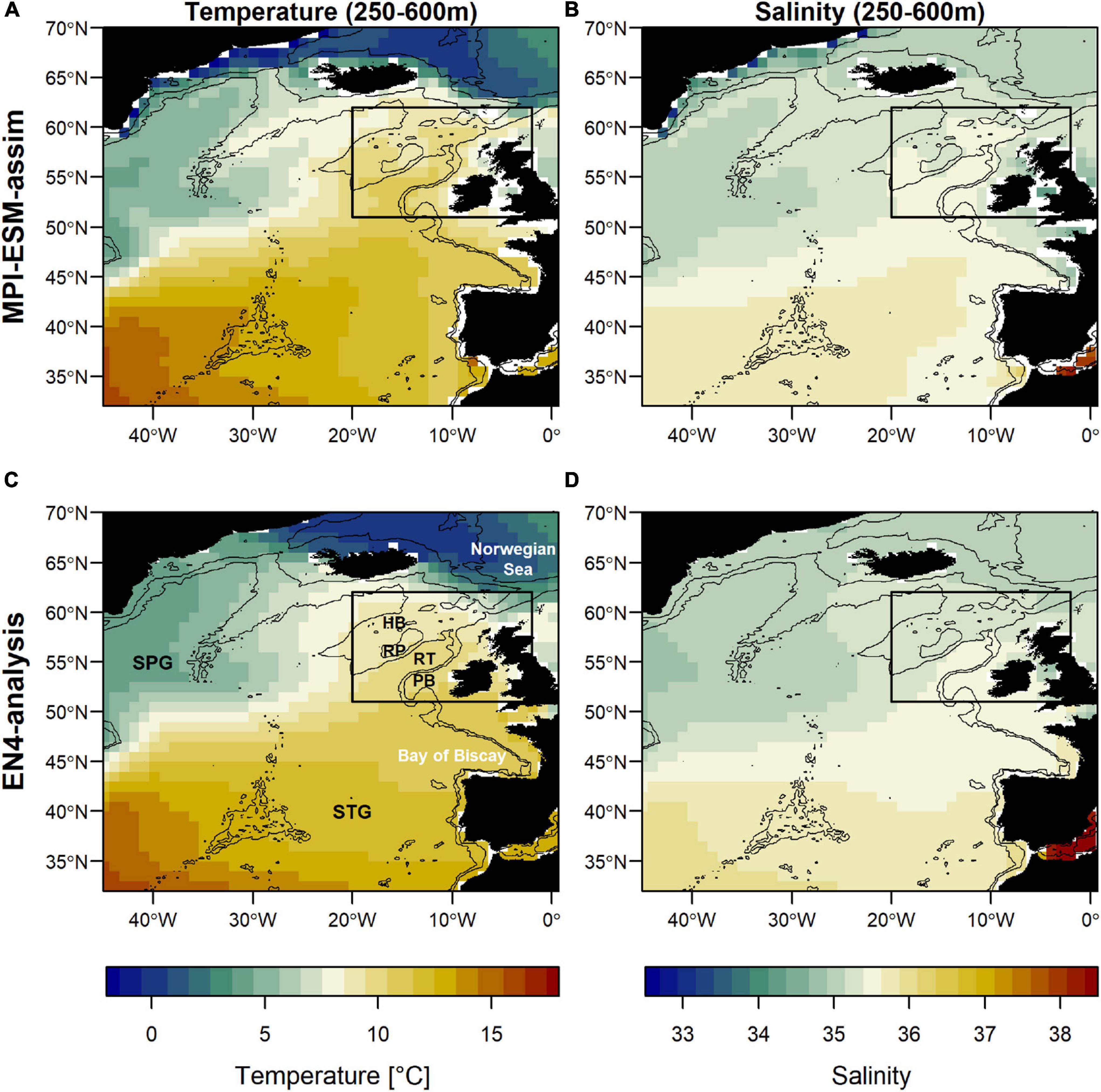
Figure 1. Mean oceanographic conditions in February, March and April (FMA; climatology of 1965–2016) within the spawning depth of blue whiting (250–600m) in terms of temperature (left; A,C) and salinity (right; B,D) for MPI-ESM-assim (top; A,B) and EN4-analysis (bottom; C,D). The black rectangle delineates the study area: the spawning region of blue whiting. Labels in panel (C) show the geographic features Hatton Bank (HB), Rockall Plateau (RP), Rockall Trough (RT), Porcupine Bank (PB), and the two dominant gyre systems North Atlantic subpolar gyre (SPG) and the subtropical gyre (STG). Bathymetry is indicated by 600 and 2000 m isobaths.
Forecasting spatial changes of the spawning distribution could also be useful for the monitoring and management of blue whiting. Every spring the International Blue Whiting Spawning Stock (IBWSS) survey samples the core spawning region of blue whiting (ICES, 2015). However, sampling is particularly challenging on RHP due to great distance to the ports and frequent bad weather conditions (ICES, 2010). Therefore, forecasting blue whiting in its spawning region with a special focus on RHP (e.g., whether spawning is going to take place on RHP) could be valuable for the IBWSS planning group (pers. communication with Jan Arge Jacobsen, member of the ICES Working Group of International Pelagic Surveys, Faroe Marine Research Institute). Accordingly, a forecast at interannual to multiannual timescales could be used as an objective decision-making tool to adjust the IBWSS survey coverage on RHP.
Forecasting the spatial distribution of marine organisms is related to the theory of the ecological niche or suitable habitat of a species (Payne et al., 2017). Previous work established the mechanistic link between the marine climate (i.e., salinity) and the spawning distribution of blue whiting based on species distribution modelling (Miesner and Payne, 2018). Species distribution models (SDMs) are also termed ecological niche models or habitat models, and represent a common method to define the suitable (i.e., potential) habitat of a species by means of correlative models that link species distribution data with environmental observations (Elith and Leathwick, 2009; Wiens et al., 2009). The suitable habitat of a species is commonly used as a proxy for its spatial distribution and applied in marine ecological forecasts such as for the spatial management of southern bluefin tuna in Australian waters (Hobday and Hartmann, 2006; Eveson et al., 2015), or Pacific sardine in Californian waters (Kaplan et al., 2016; Siedlecki et al., 2016).
Based on the previously developed SDM (Miesner and Payne, 2018) and persistence of salinity, first attempts to operationalise a forecast of the suitable spawning habitat of blue have been undertaken (ICES, 2018; Payne and Lehodey, 2019) and are currently provided two months prior to the IBWSS survey (Payne, 2021). However, due to the highly variable nature of the marine environment, the management of living marine resources, such as fish, challenges the stationary assumption in persistence forecasts (Tommasi et al., 2017a). The oceanographic conditions in the spawning region of blue whiting are characterised by a mixture of warm and saline subtropical Eastern North Atlantic Water coming from the south and cool and fresh subpolar Western North Atlantic Waters from the north (Holliday et al., 2000; Hátún et al., 2009a). The relative mixture of these water masses is related to changes in the North Atlantic Subpolar Gyre (SPG) and creates a distinct marine climatic regime to which blue whiting respond through changes in their spatial distribution (Hátún et al., 2009b; Miesner and Payne, 2018). Generally, a strong SPG leads to fresher and cooler conditions in the spawning region, causing blue whiting to cluster along the continental shelf (Hátún et al., 2009b). A weak SPG promotes more saline and warm subtropical water masses which leads to a westward expansion of the spawning distribution onto Rockall Plateau and Hatton Bank (Figure 1; Hátún et al., 2009b; Miesner and Payne, 2018). A modelling study based on blue whiting larvae found that spawning is confined to a certain range of salinity and proposed that this link could form the basis of forecasting changes in the spawning distribution of blue whiting (Miesner and Payne, 2018). The dynamics of the SPG have been shown to be well represented in the dynamic coupled Max Planck Institute Earth System Model (MPI-ESM; Koul et al., 2019). Accordingly, we explore the potential for developing a forecast of the suitable spawning habitat of blue whiting based on annual to multi-annual time scales with MPI-ESM, which could be valuable for both augmenting monitoring surveys, and enhancing long-term management of the species.
In the first part of the study, we assess whether the marine climate, i.e., temperature and salinity, is predictable within the region and depth at which blue whiting spawn during the months of spawning. We judge the quality of the MPI-ESM hindcast by comparing it to two reference data sets: the EN4 objective analysis (Good et al., 2013) and the MPI-ESM ensemble Kalman filter assimilation (Polkova et al., 2019; Brune and Baehr, 2020). In the second part of the study, we analyse two ways to extract information on the suitable spawning habitat from SDMs and explore the potential of forecasting the suitable spawning habitat of blue whiting up to five years ahead.
Materials and Methods
Modelling and Analysis Strategy
We analyse the skill of 5-year predictions of the marine climate and subsequently of the suitable spawning habitat of blue whiting. These are based on decadal retrospective forecasts, in the following called hindcasts, of the dynamical state of the ocean with MPI-ESM (Polkova et al., 2019; Brune and Baehr, 2020). In the first part of the study, we analyse whether we can make skilful predictions of the marine climate with the MPI-ESM hindcast at spatial and temporal scales relevant for spawning blue whiting. We assess the quality of the hindcast by comparison to two reference products: the EN4 objective analysis (Good et al., 2013) and the MPI-ESM ensemble Kalman filter assimilation (Polkova et al., 2019; Brune and Baehr, 2020), hereafter referred to as EN4-analysis and MPI-ESM-assim, respectively (Figure 2.1).
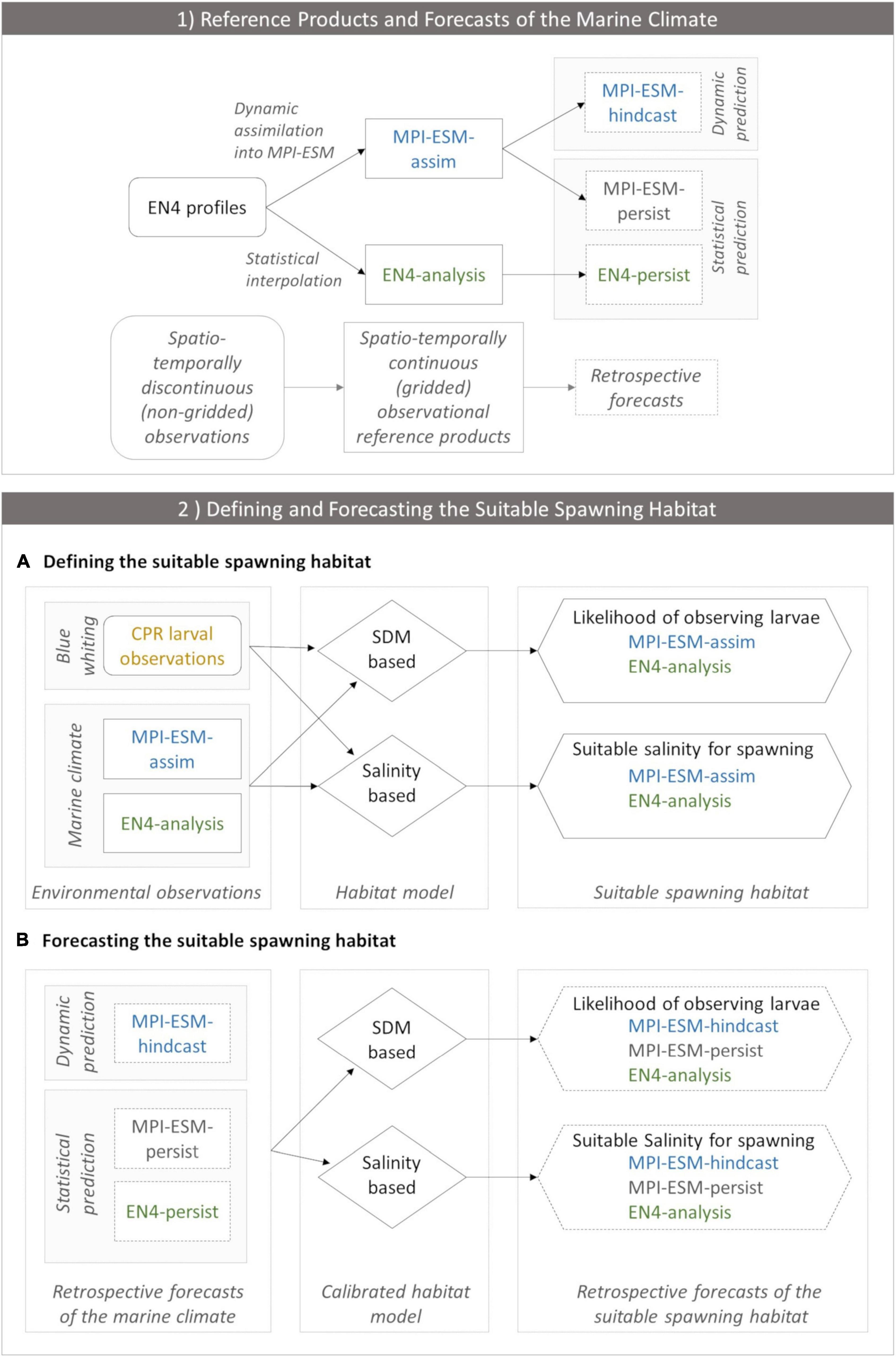
Figure 2. (1) Observational reference products of the marine climate (EN4-analysis and MPI-ESM-assim; solid boxes) and the corresponding retrospective forecasts (dashed lines) employed in the study and (2) the workflow of defining (A) and forecasting (B) the suitable spawning habitat of blue whiting. In panel (1) EN4 profiles (rounded box) contain spatio-temporally discontinuous (non-gridded) observations of the marine climate. In order to create spatio-temporally continuous (gridded) observational reference products, either EN4 profiles are assimilated into MPI-ESM resulting in MPI-ESM-assim or EN4 profiles are statistically interpolated forming the EN4-analysis. Thereby, both MPI-ESM-assim and EN4-analysis contain the same non-gridded oceanographic observations (EN4 profiles) but their methods to close observational gaps differ. These observational reference products form the basis for retrospective forecasts of the marine climate. MPI-ESM-assim forms the basis for the dynamic prediction system MPI-ESM-hindcast. Moreover, MPI-ESM-assim and EN4-analysis are employed to form the statistical persistence forecasts MPI-ESM-persist and EN4-persist, respectively. (2) Workflow of defining (A) and forecasting (B) the suitable spawning habitat of blue whiting, indicating how input data (rectangles) feeds into each habitat model (rhombus) which transform this information into approximations of the suitable spawning habitat (hexagon). (A) Environmental observations include CPR larval observations of blue whiting (yellow) and information from the marine climate from either MPI-ESM-assim (blue) or EN4-analysis (green). These environmental observations calibrate each habitat model. The SDM translates this information into the likelihood of observing larvae for MPI-ESM-assim and EN4-analysis, respectively, which is a probabilistic proxy for the suitable spawning habitat. The salinity based habitat model transforms the environmental observations into the suitable salinity for spawning for MPI-ESM-assim and EN4-analysis, respectively, which forms a deterministic proxy for the suitable spawning habitat. (B) Forecasts of the suitable spawning habitat are based on retrospective forecasts of the marine climate (dashed rectangles) which includes one dynamic prediction system (MPI-ESM-hindcast; blue) and two statistical predictions (MPI-ESM-persist or EN4-persist; grey and green, respectively). Each retrospective forecast of the marine climate feeds into a calibrated habitat model (either the SDM or salinity based), which transforms this information into retrospective forecasts of the suitable spawning habitat (either in terms of the likelihood of observing larvae for the SDM based habitat model, or the suitable salinity for spawning).
The spatially complete EN4-analysis provides one way of filling the gaps between sparsely observed oceanic profiles using iterative optimal interpolation (Good et al., 2013). Another approach is used by MPI-ESM-assim, where EN4 profiles are incorporated into the ocean model component of a dynamic ESM. We are aware that, strictly speaking, MPI-ESM-assim and MPI-ESM-hindcast may not be totally independent. Nevertheless, assimilations with MPI-ESM can be used to overcome the problem that oceanic observations insufficiently sample the oceanic state, and to create a consistent reference state (Brune et al., 2015; Brune and Baehr, 2020). Both our reference products rely on EN4 profiles. We therefore expect that the considerable increase in the number of profiles after 2001 with the Argo program decreases the uncertainty in our reference products after 2001. Finally, the predictive skill of the hindcast is assessed retrospectively by comparison to reference forecasts based on EN4-analysis and MPI-ESM-assim persistence.
In the second part of the study, we analyse whether we can make skilful predictions of the suitable spawning habitat of blue whiting (a workflow of this approach is presented in Figure 2.2). We explore two ways to extract information on the suitable spawning habitat from SDMs. While we create novel SDMs based on either MPI-ESM-assim or EN4-analysis in the first approach, the second method employs the salinity defined as suitable for spawning by Miesner and Payne (2018) to delineate the suitable spawning habitat. The approach that is superior in representing the observed spawning distribution of blue whiting is subsequently employed for the creation of coupled physical-biological forecasts. Here, the suitable spawning habitat of blue whiting is forecasted retrospectively based on the MPI-ESM hindcast and two persistence forecast and their predictive skill is judged against fishery and survey observation.
Study Region and Time Period of Interest
The study region covers the core spawning area of blue whiting west of the British Isles which is sampled annually by the ICES IBWSS survey (ICES, 2015): 20°W to 2°W and 51°N to 62°N (black rectangle in Figure 1) and will henceforth be referred to as spawning region. We define RHP by the local bathymetry, following the 1,000 m depth isobath around Rockall Plateau, George Bligh Bank and Hatton Bank finishing west at the border of the IBWSS sampling region. To encompass the depth range where eggs, non-feeding larvae and spawning adults have been observed (Coombs et al., 1981; Hillgruber and Kloppmann, 1999; Ådlandsvik et al., 2001), we define the spawning depth of blue whiting between 250 and 600 m. The main spawning activity of blue whiting takes place during late March and early April which corresponds to the timing of the IBWSS survey (Bailey, 1982; ICES, 2015). Since blue whiting larvae are observed in the surface waters mainly between March and May with a peak in April (Pointin and Payne, 2014; Miesner and Payne, 2018) and need around 3 weeks for the ascent to the surface (Ådlandsvik et al., 2001), it is likely that spawning ranges from February to April.
Accordingly, the average temperate and salinity between February and April (FMA) at 250 to 600 m depth within the spawning region of blue whiting resembles the oceanographic conditions, i.e., the marine climate, experienced by the spawning adults and the larvae.
Observations and Retrospective Forecasts of Temperature and Salinity
Observations of Temperature and Salinity
Monthly observations of ocean temperature and salinity are available from the Met Office Hadley Centre’s EN4 data set (Good et al., 2013). Besides quality controlled in situ profiles, hereafter termed EN4 profiles, a spatially comprehensive objective analysis is available which uses an iterative optimal interpolation to fill all observational gaps. We use the EN4 objective analysis version 4.2.1 with corrections based on Gouretski and Reseghetti (2010), which is available from 1900 to the present and contains 42 vertical levels and a regular 1° horizontal resolution (Good et al., 2013) and will be referred to as EN4-analysis. We select the period 1958–2016 and average yearly FMA-mean values of temperature and salinity vertically over 252–596 m to characterise the marine climate in the spawning region and depth of blue whiting.
Assimilation and Dynamical Hindcasts of Temperature and Salinity
Another way of creating a spatially complete data set that serves as a good estimate of the true state of the ocean, is to incorporate (i.e., assimilate) oceanic observations into a coupled ocean-atmosphere model. We use an experiment from the Max Planck Institute ESM at low resolution (MPI-ESM; Giorgetta et al., 2013). Its ocean component (Jungclaus et al., 2013) contains 40 levels and has an effective resolution of around 0.6°–0.9° (67–100 km) within the spawning region. Monthly observations of oceanic temperature and salinity from EN4 profiles (Good et al., 2013) are assimilated into MPI-ESM using a full-value 16-member ensemble Kalman filter (EnKF) approach (Polkova et al., 2019; Brune and Baehr, 2020). Additionally, the dynamical state of the atmospheric component is nudged toward ERA40/ERAInterim reanalyses from ECMWF (Uppala et al., 2005; Dee et al., 2011), and external forcings of the Phase 5 Coupled Model Intercomparison Project (CMIP5) were applied (Taylor et al., 2012). We run MPI-ESM with these settings from 1958 to 2016 and simulate an assimilation which will henceforth be referred to as MPI-ESM-assim. Thereby, MPI-ESM-assim dynamically represents observed temperature and salinity in a model-consistent way (Brune and Baehr, 2020).
Based on MPI-ESM-assim, a 16-member hindcast ensemble is created (Brune and Baehr, 2020), which will be referred to as MPI-ESM-hindcast. MPI-ESM-hindcast is initialised every year from the 1st of November 1960 to 2016. In this study, each initialisation is running for 5 years. The time counting from the initialisation date of the hindcast is termed lead time. Accordingly, if the initialisation date is November 1960 and the hindcast is for March (or FMA) 1961, the (mean) lead time is 4 months and within lead year 1, while a hindcast for March (or FMA) 1962 has a lead time of (around) 1 year and 4 months, or within lead year 2.
We regrid both MPI-ESM-assim and MPI-ESM-hindcast to a 1° × 1° regular grid and create the average of the 16 ensemble members (i.e., the ensemble mean) which we analyse throughout the study. For MPI-ESM-assim and MPI-ESM-hindcast we average annual FMA-mean values of temperature and salinity vertically between 240 and 600 m to derive the environmental conditions within the spawning depth of blue whiting.
Persistence Forecast
Persistence forecasts are a common reference in seasonal to decadal forecasting used to judge the skill of a hindcast: hindcasts which outperform persistence exemplify the benefit of using a dynamic ESM (Wilks, 2011; Jolliffe and Stephenson, 2012). Persistence forecasts presume that future conditions are equal to past conditions, e.g., a persistence forecast of FMA in 1965 with a lead time of two years, uses observations of FMA in 1963 as a forecast by assuming stationarity for the duration of the forecast (i.e., 2 years). We create persistence forecasts for EN4-analysis and MPI-ESM-assim for five lead years, termed EN4-persist and MPI-ESM-persist, respectively.
Predictability of Temperature and Salinity Within the Spawning Region of Blue Whiting
Here, we compare retrospective forecasts (i.e., MPI-ESM-hindcast, MPI-ESM-persist and EN4-persist) to MPI-ESM-assim and EN4-analysis, by means of the anomaly correlation coefficient (ACC) and the root-mean squared error (RMSE) which are common measures of forecast accuracy (Wilks, 2011; Jolliffe and Stephenson, 2012). We calculate anomalies based on the mean temperature and salinity of the common time period (1965–2016; e.g., FMA 1965 minus mean FMA from 1965 to 2016). In order to remove the influence of long-term trends on the prediction we linearly detrend the time series before calculating the skill. To account for the uncertainty in predictive skill, we perform a bootstrap with 500 iterations of ACC and RMSE for the common time period (the years 1965–2016 are shuffled 500 times with replacement and the ACC/RMSE calculated for each lead year). Significance of the ACC is defined from the 95% confidence interval of the bootstrap. Throughout the study, we show the median ACC and RMSE.
To analyse prediction skill over lead time the detrended anomalies are averaged over the study region and ACC and RMSE calculated. For this, the mean bias between forecast and observation is calculated and subtracted from the forecast for each year before RMSE and ACC are calculated from the respective time series. The confidence interval calculated from the bootstrap is defined as the interquartile range between the lower quartile (25th percentile) and the upper quartile (75th percentile) of the bootstrapped data. For the spatial representation of predictive skill, ACC and RMSE are calculated for each grid point where water depth exceeds 600 m. Water depth is based on NOAAs ETOPO1 product (Amante and Eakins, 2009).
Forecasting the Suitable Spawning Habitat of Blue Whiting Retrospectively
Retrospective Forecasts Based on SDMs
We create novel SDMs with observations of blue whiting larvae from the Continuous Plankton Recorder (CPR) survey (Reid et al., 2003) obtained from the Marine Biological Association in Plymouth. The probability of observing blue whiting larvae is modelled as a function of a fixed geographical model component, including latitude and the day-of-the-year, bathymetry, the solar elevation angle and varying environmental variables (Table 3) using Generalised Additive Models (Wood, 2006) analogous to Miesner and Payne (2018). Thus, the SDM accounts for the meridional migration of adults (Bailey, 1982) and the diel vertical migration of larvae (Hillgruber and Kloppmann, 2000) which can affect the capture efficiency of the CPR (Pointin and Payne, 2014). The environmental variables consist of temperature and salinity, since these are predictable with ESMs.
We create two sets of SDMs: one calibrated with environmental data from EN4-analysis and another one calibrated with MPI-ESM-assim, in order to account for the difference in these products in handling the spatially incomplete EN4 profiles. We calculate the salinity and temperature at the spawning depth of blue whiting during the time of spawning (SSPAWN and TSPAWN), i.e., one month prior to a CPR observation (Miesner and Payne, 2018), by averaging vertically over 252–596 m for EN4 and 240–600 m for MPI-ESM, since the depth layers slightly vary between the two. At locations where water depth is shallower than 252 m for EN4-analysis or shallower than 240 m for MPI-ESM, we select variables closest to the seafloor. In order for the SDMs to be comparable, we couple the same CPR observations to EN4-analysis and MPI-ESM-assim, containing 48 years from 1958 to 2005 including 68,229 observations with 938 presences of blue whiting larvae. The resulting spatial distribution of larval-presence probability can be understood as a proxy for the suitable spawning habitat of blue whiting (Miesner and Payne, 2018).
Validation of the SDM and model selection is in line with Miesner and Payne (2018). As a primary metric for model selection, we choose the Akaike Information Criteria (AIC); Anderson, 2008; Burnham et al., 2011). The explained deviance is equivalent to the coefficient of determination (R2) and considered an overall indicator of model quality.
We derive the capability of the models to distinguish between the presence and absence of larvae from a contingency table (Table 1). We convert the predicted probability of blue whiting larval-occurrence from the SDM into presences and absences by selecting the threshold so that the total number of presences in the prediction data set is equal to the number of presences in the observed dataset, in accordance with Freeman and Moisen (2008). Moreover, we calculate mean values of the true skill statistic (TSS), positive predictive value (PPV), and negative predictive value (NPV) based on four-fold cross validation with 75% of the data used for training and the remaining for validation, with every 4th year included in one fold (Table 2; see also Liu et al., 2011; Jolliffe and Stephenson, 2012). Additionally, we consider the area under the receiver operating characteristic curve (AUC), which relates the relative proportions of correctly and incorrectly classified predictions (HR and FAR, respectively) over a range of threshold levels (Brown and Davis, 2006; Liu et al., 2011).
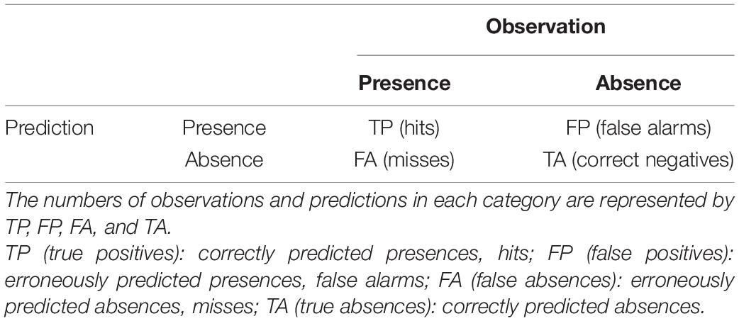
Table 1. Contingency table used to evaluate the predictive accuracy of binary events.
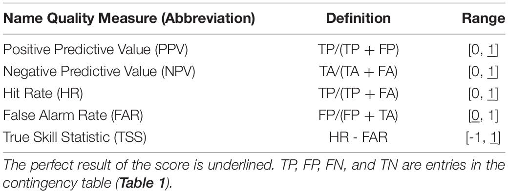
Table 2. Verification Scores.
We base the choice of the best performing SDM on two steps. First we create a subset for each of the two SDM sets (one calibrated with EN4-analysis and the other with MPI-ESM-assim) with all models having AIC differences smaller than 15 (Table 3), since models with an AIC difference larger than 15 are considered to be very dissimilar (Anderson, 2008). From these subsets, we select the SDM with the highest predictive performance in terms of TSS, PPV, NPV, and AUC as the “best” performing model and analyse it further.
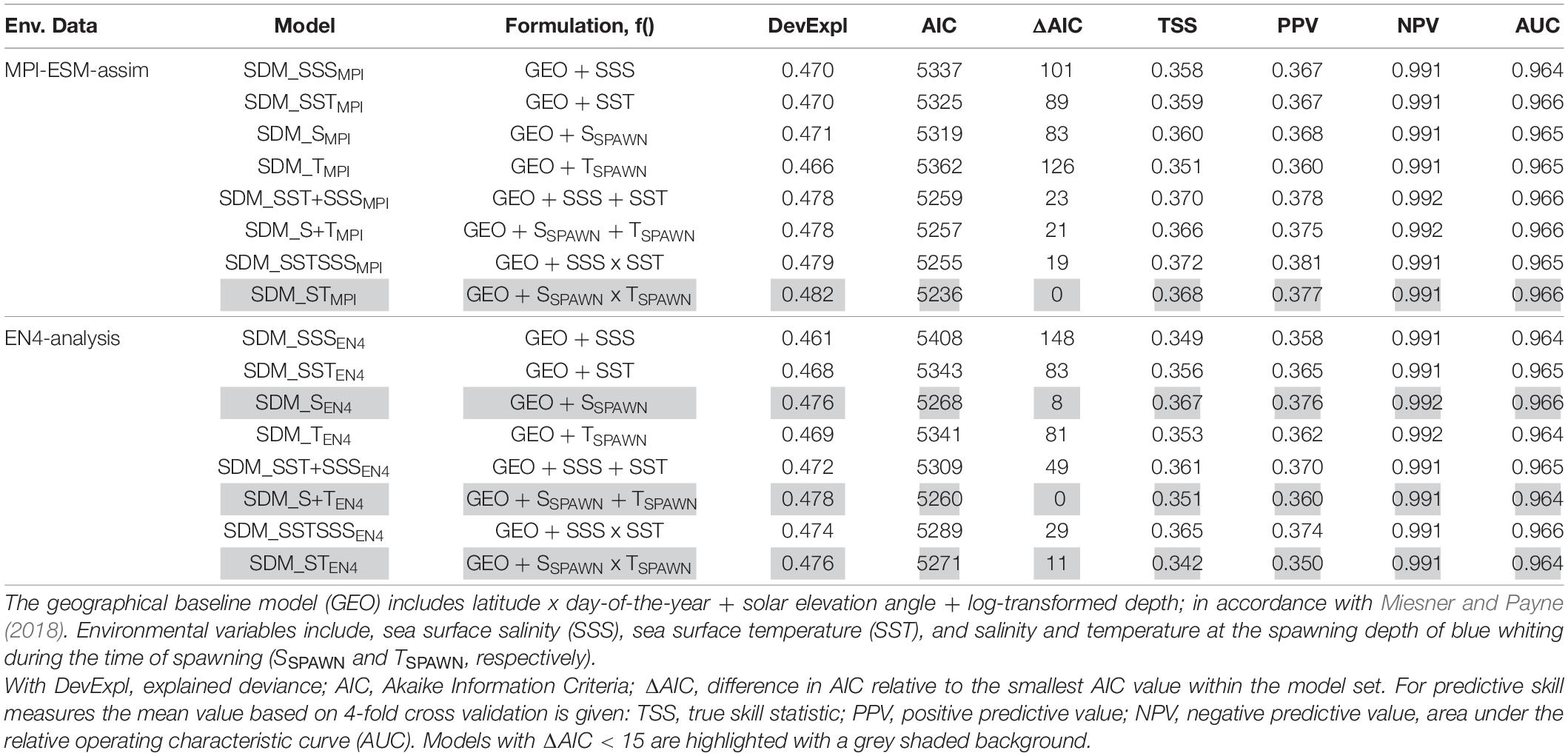
Table 3. Model fitting results for species distribution models (SDM) calibrated with different environmental reference data (Env. Data).
We create retrospective forecasts of the suitable spawning habitat by coupling the best performing SDMs (Table 3) to retrospective forecast of the marine climate for up to five lead years. Specifically, we employ the best performing SDM calibrated with MPI-ESM-assim for retrospective forecasts based on MPI-ESM-hindcast and MPI-ESM-persist. While we use the best performing SDM fitted to EN4-analysis for retrospective forecasts based on EN4-persist. Within the SDM, we select the 15th of each month as the day-of-year owing to the monthly resolution of environmental data and fix the solar elevation angle to 0°, representative of sunrise or sunset, in line with Miesner and Payne (2018). SDMs are calibrated with full-value temperature and salinity data (i.e., not anomalies) from MPI-ESM-assim and EN4-analysis, respectively, and transform this information into blue whiting larval presence probability. Therefore, forecasts based on SDMs are directly comparable and there is no need for bias correction.
Retrospective Forecasts Based on Salinity
As an alternative approach to creating new SDMs, solely the suitable salinity for spawning is used as a proxy for the suitable spawning habitat. A previous study based on SDMs, observations from the CPR and an earlier version of the EN4 objective analysis (EN4.1.1) showed a dome-shaped relationship between salinity (SSPAWN) and the probability of observing blue whiting larvae with a non-zero likelihood of observing larvae at salinities between 35.28 and 35.53 (Miesner and Payne, 2018: SDM 3, Table 4 and Figure 9). This suitable salinity for spawning corresponded well to independent observations from both fishery and scientific surveys (Miesner and Payne, 2018) and is in line with the re-calibrated SDM based on EN4-analysis that is applied in this study (SDM_SEN4).
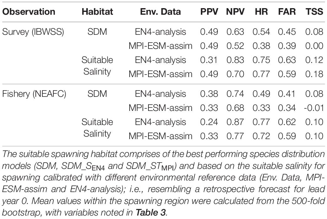
Table 4. Agreement of the suitable spawning habitat with independent observations of adult blue whiting observed in the IBWSS survey and caught in fishery (NEAFC) during March and April within the spawning region.
The suitable salinity for spawning in MPI-ESM is bias-corrected to offset the mean deviations between MPI-ESM-assim and EN4-analysis within the spawning region and during the time period for which validation data is available (0.06 for 1977–2012). Retrospective forecasts of the suitable salinity for spawning are based on full-value retrospective forecasts of salinity with MPI-ESM-hindcast, MPI-ESM-persist and EN4-persist. The respective isohaline where the salinity is defined suitable is used as a proxy for defining those grid cells in our simulation, which are deemed to cover the suitable spawning habitat.
Observations of Adult Blue Whiting
The first data set comprises of acoustic surveys of blue whiting spawning aggregations from 1981 to 2013, spanning 25 years due to incomplete time series. Before 2004 the observations were solely based on Norwegian surveys of the spawning stock, while data from 2004 onward originate from the from the IBWSS survey that is carried out annually for 2 weeks from late March to early April (ICES, 2016). The survey records acoustic data continuously along its cruise tracks and provides estimates of blue whiting biomass. While most years had a resolution of 0.5° latitude × 1° longitude, the data resolution is coarser for the period 2002–2006 with 1° latitude × 2° longitude.
The second set of independent observations consists of monthly fishery catch statistics of blue whiting from 1977 to 2012 from the NEAFC (2013) targeting spawning adults with a resolution of 0.5° latitude × 1° longitude. The fishery data is averaged over March and April, in congruence with the IBWSS survey data.
For both, the survey and the fishery data, the grid cells within the spawning region where blue whiting were observed or caught are treated as presence. All remaining cells are treated as absences, since absences of fish are hardly reported in catch statistics (e.g., for the months March and April only 0.1% of the available fisheries data within the spawning region were absences) and are also low in the survey (0.9% within the spawning region). Therefore, including the absence data would render the observations unfit for model- and forecast evaluation.
Predictive Skill of the Suitable Spawning Habitat Forecast
Observations of adult blue whiting in March and April are compared to retrospective forecasts of blue whiting’s suitable spawning habitat averaged over March and April and for each lead year (0–5) using binary verification metrics based on the contingency table (Table 1). Accordingly, the output of the biological forecasts are brought to the same spatial grid as the observations (0.5° latitude × 1° longitude). Predicted presence-probabilities from the SDM are converted into presence and absence by selecting the threshold where predicted prevalence from the SDM is equal to observed prevalence (Freeman and Moisen, 2008). For the salinity based forecast, each grid cell within the range of the suitable salinity for spawning is defined as presence (of suitable habitat) and the remaining as absence.
We quantify predictability via TSS, the difference between Hit Rate and False Alarm Rate (Table 2). A TSS of 1 indicates that the forecast’s accuracy is perfect, and a TSS of zero is associated with a purely random forecast (Table 2). In each grid point, all entries of the contingency table must be sufficiently filled for our analysis to be robust and viable. To ensure statistical reliability, we prescribe this condition for each 500-fold bootstrap iteration. In practice, the counts of true presences (TP) and false absences (FA) are the critical indicators. Thus, we neglect grid-cells when the sum of both critical indicators is equal to zero in at least one bootstrap iteration.
First, we evaluate both definitions of the suitable spawning habitat against fishery and survey data. Afterward, we select retrospective forecasts of the suitable spawning habitat at lead year 0 with best observational agreement in terms of TSS for more detailed analysis.
We analyse the predictive skill at RHP by pooling the bootstrapped forecast verification metrics (i.e., TSS) for each lead year over this region (averaging 40 and 46 grid cells for the survey and the fishery data, respectively). Uncertainty is expressed in terms of the interquartile range between the lower quartile (25th percentile) and the upper quartile (75th percentile) of the bootstrapped data. We define significance of the TSS by the 95% confidence interval of the bootstrap.
In order to analyse inter-annual variations in skill, we calculate the annually TSS averaged over RHP for retrospective forecasts made approximately one year ahead. Due to the different initialisation dates we compare MPI-ESM-hindcast with a lead time of around 16 months (lead year 2) to persistence forecasts at 12 months lead (lead year 1 for EN4-persist and MPI-ESM-persist).
The Suitable Spawning Habitat as an Indicator for Spawning on Rockall-Hatton Plateau
Finally, we evaluate whether retrospective forecast of the suitable spawning habitat can be applied to anticipate whether spawning takes place on RHP. For each year, the spatial coverage of blue whiting observations on RHP is calculated as the percentage of grid cells within RHP containing presences of blue whiting from fishery/survey observations in March and April. Likewise, the percentage of grid cells within RHP containing suitable habitat in RHP is calculated for each year in March and April, based on retrospective forecasts with MPI-ESM-hindcast for lead year 2 (16 months ahead) and persistence forecasts for lead year one (12 months ahead) with EN4-persist and MPI-ESM-persist.
Results
Representations of the Marine Climate in EN4-Analysis and MPI-ESM-Assim
The large-scale features of temperature and salinity from February to April (FMA) are similar in MPI-ESM-assim and EN4-analysis within the spawning depth of blue whiting (250–600 m; Figure 1). However, on smaller scales (e.g., RP, RT), MPI-ESM-assim and EN4-analysis differ. Within the spawning region and spawning depth of blue whiting, anomalies of temperature agree well in EN4-analysis and MPI-ESM-assim (overall correlation in FMA of 0.85, bias 0.66°C; Figure 3A), while differences are more pronounced in terms of salinity (correlation 0.51; bias 0.08; Figure 3B). EN4-analysis and MPI-ESM-assim show similar temporal deviations from climatology and multi-decadal variability in both temperature and salinity. Both observational products show more saline and warmer water up to the 1970s and rather low anomalies around 1975 and from 1986 to around 1995, followed by an increase up to around 2010 and a stark decrease in subsequent years, again in line with observations from the eastern Ellet Line around Rockall Plateau (Holliday et al., 2015, 2020). During some periods, e.g., around 1965 and 1995 there is a tendency of MPI-ESM-assim to show a higher amplitude of deviations in terms of salinity than EN4-analysis (Figure 3B). Deviations from climatology are less pronounced for MPI-ESM-hindcast, as shown for lead year 2, in particular for salinity during the past 20 years of the study period (Figure 3B).
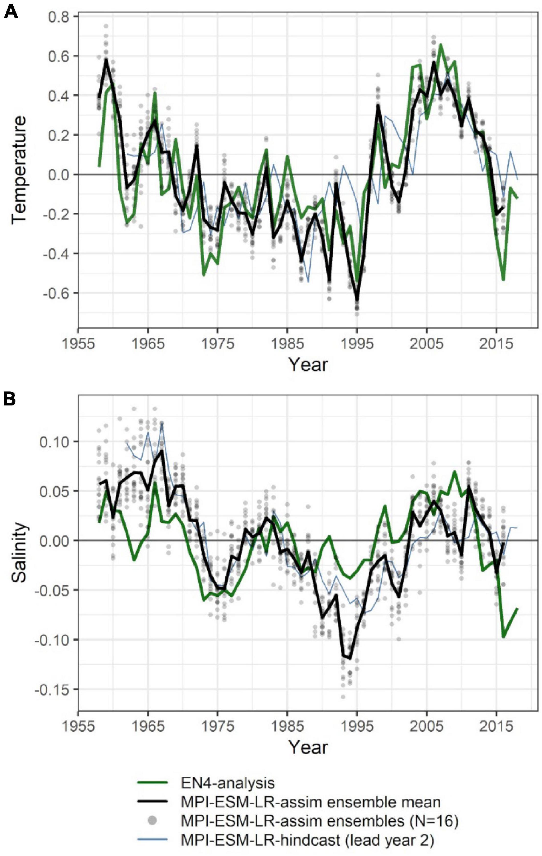
Figure 3. Mean FMA temperature (A) and salinity (B) anomalies averaged over the spawning depth of blue whiting (250–600 m) within the spawning region (black rectangle in Figure 1). Data from EN4-analysis is indicated by the green line. The ensemble mean of the assimilation run of MPI-ESM (MPI-ESM-assim) is indicated by the black line and its individual ensembles are shown as grey dots, where overlapping ensembles create darker shades. MPI-ESM-hindcast of lead year 2 is added as blue line.
Predictive Skill of the Marine Climate
Within the spawning region of blue whiting, MPI-ESM-hindcast shows greater predictive skill for salinity compared to temperature and is more skilful than MPI-ESM-persist, when compared to MPI-ESM-assim (Figure 4). The salinity within the spawning region and spawning depth can skilfully be predicted for more than 4 years ahead (Figures 4B,D). In terms of the ACC, the hindcast of salinity outperforms persistence for all analysed lead years (Figure 4B), while the predictive skill of temperature is similar to persistence and degrades further after lead year 3 (Figure 4A). Moreover, salinity is more predictable than temperature, with a median ACC above 0.6 for all lead years analysed (Figures 4A,B). In terms of the RMSE MPI-ESM-hindcast is more skilful than MPI-ESM-persist in predicting both temperature and salinity, with most pronounced differences for temperature (Figures 4C,D), indicating that the hindcast is superior in representing the amplitude of observed variations in salinity, and in particular temperature. The RMSE of the persistence forecasts increases with increasing lead times, while the RMSE is rather constant for the hindcast from lead year 2 onward, indicating a greater accuracy of the hindcast with increasing lead times compared to persistence. Comparing MPI-ESM-hindcast to EN4-analysis shows a similar pattern for temperature; however, MPI-ESM-hindcast shows for salinity has a higher uncertainty and outperforms EN4-persist only after lead year 3 (Figure 5). Overall, the predictive skill of MPI-ESM-persist (Figure 4) and EN4-persist (Figure 5) is nearly identical and both show slightly higher ACC for salinity than for temperature.
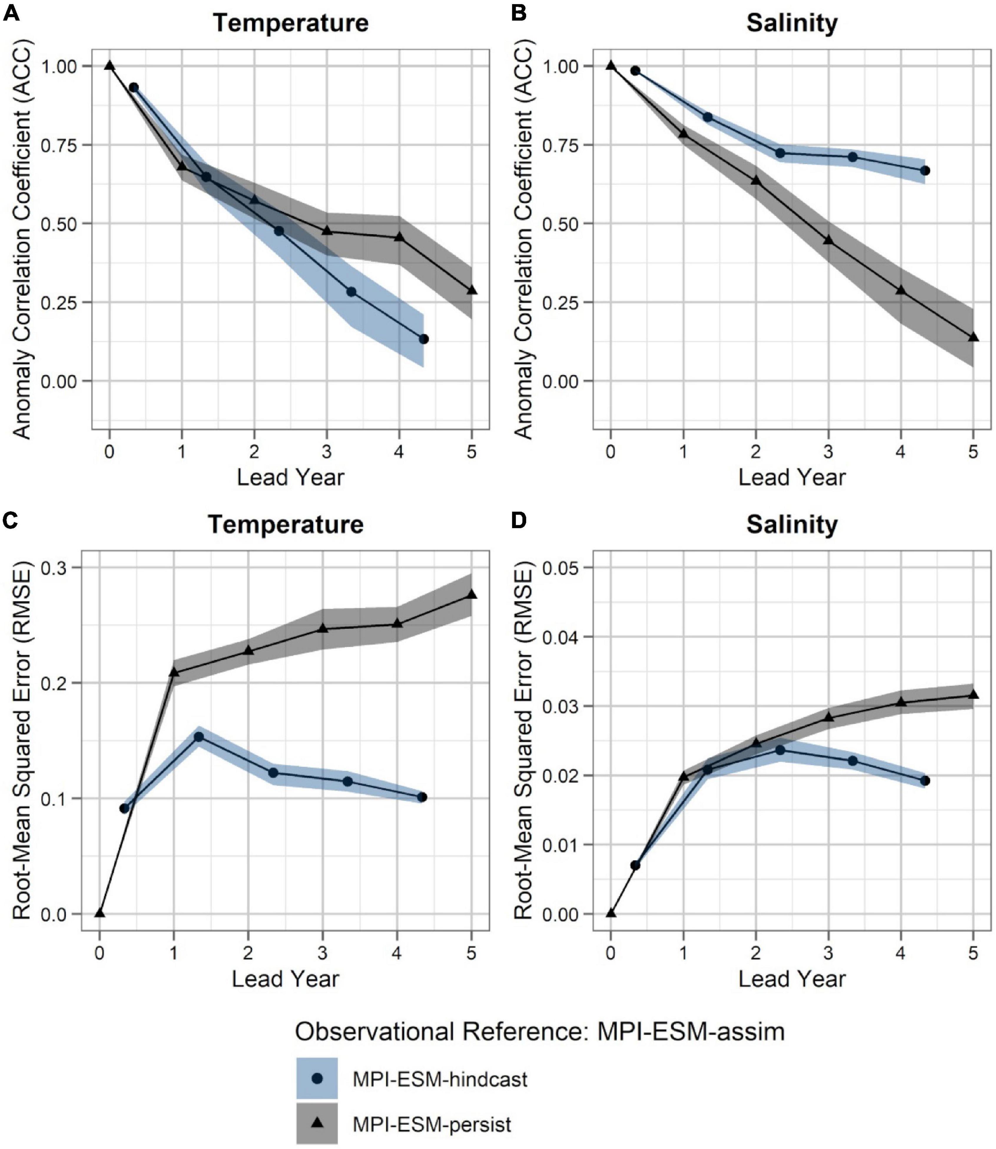
Figure 4. Predictability of temperature (left; A,C) and salinity anomalies (right; B,D) averaged over 250–600 m in FMA within the spawning region (black rectangle in Figure 1), measured in terms of the anomaly correlation coefficient (ACC; top row) and root-mean squared error (RMSE; bottom row) of MPI-ESM-hindcast (bullet; blue area) and MPI-ESM-persist (triangle; grey), judged against MPI-ESM-assim. The connected bullets/triangles indicate the median and the blue/grey shaded areas indicate spread based on the lower and the upper quartile of a 500-fold bootstrap. Two correlations (or RMSEs) are markedly different when their respective shaded areas show no overlap.
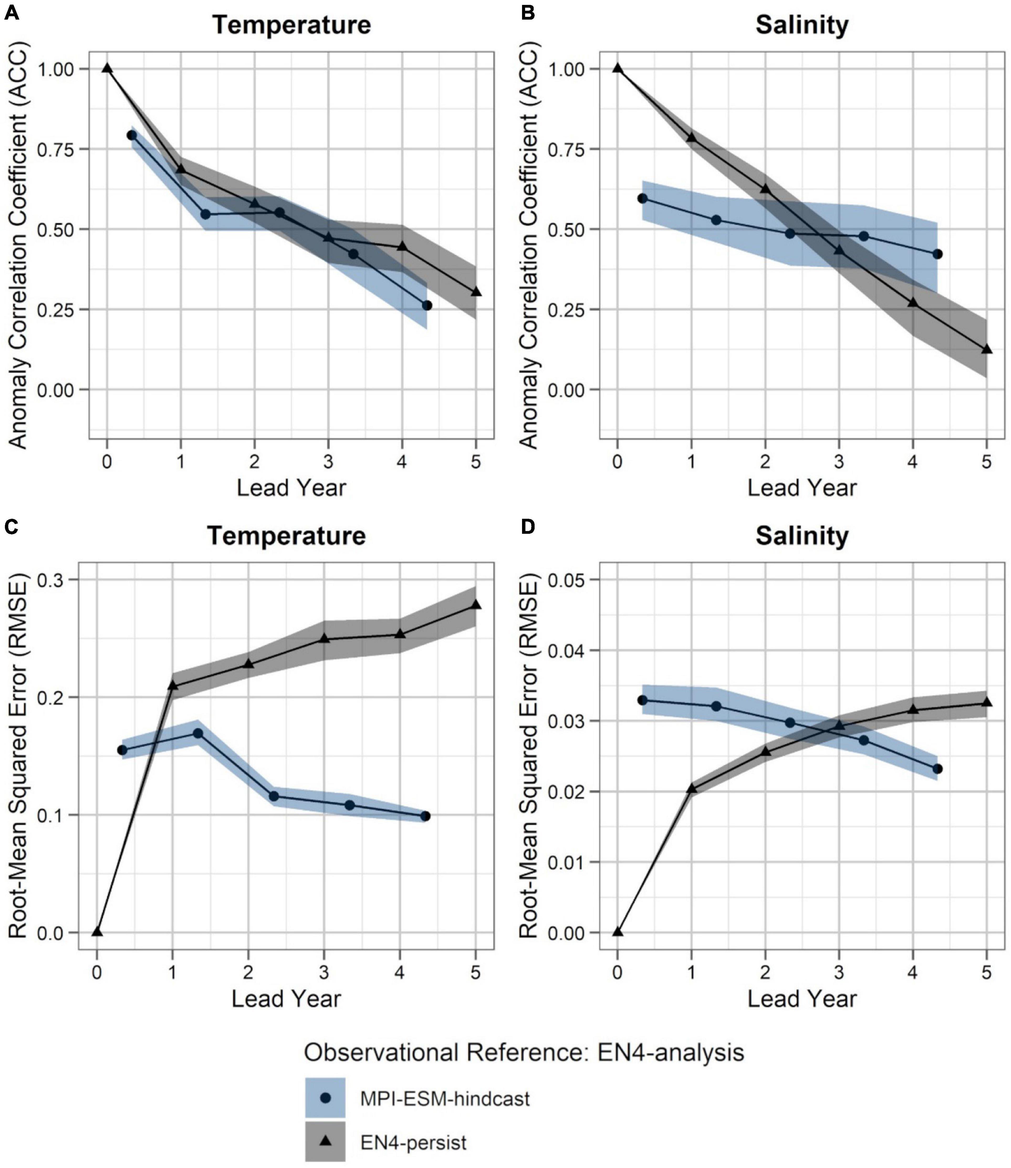
Figure 5. Predictability of temperature (left; A,C) and salinity anomalies (right; B,D) averaged over 250–600 m in FMA within the spawning region (black rectangle in Figure 1), measured in terms of the anomaly correlation coefficient (ACC; top row) and root-mean squared error (RMSE; bottom row) of MPI-ESM-hindcast (bullet; blue area) and EN4-persist (triangle; grey), judged against EN4-analysis. The connected bullets/triangles indicate the median and the blue/grey shaded areas indicate spread based on the lower and the upper quartile of a 500-fold bootstrap. Two correlations (or RMSEs) are markedly different when their respective shaded areas show no overlap.
Accordingly, considering both oceanographic reference products, a clear advantage of using MPI-ESM-hindcast in contrast to persistence is found after lead year three for salinity (Figures 4B,D, 5B,D). This indicates that salinity can skilfully be predicted with MPI-ESM-hindcast at multi-annual lead times within blue whiting’s spawning region and spawning depth during the peak months of spawning. For temperature, the hindcast is only superior in predicting the amplitude, but not the phase of observed variations, as indicated by significantly different values of RMSE but similar values of ACC when comparing persistence to MPI-EM-hindcast (Figures 4A,C, 5A,C).
There are two large regions of high predictive skill of MPI-ESM-hindcast during FMA: one in the SPG region south west of Iceland and within the STG west off the European mainland, which are separated by a region of low predictive skill entering the spawning region from the south-west (Figures 6, 7), similar to findings by Koenigk and Mikolajewicz (2009), Matei et al. (2012)Brune et al. (2018) and Frölicher et al. (2020).
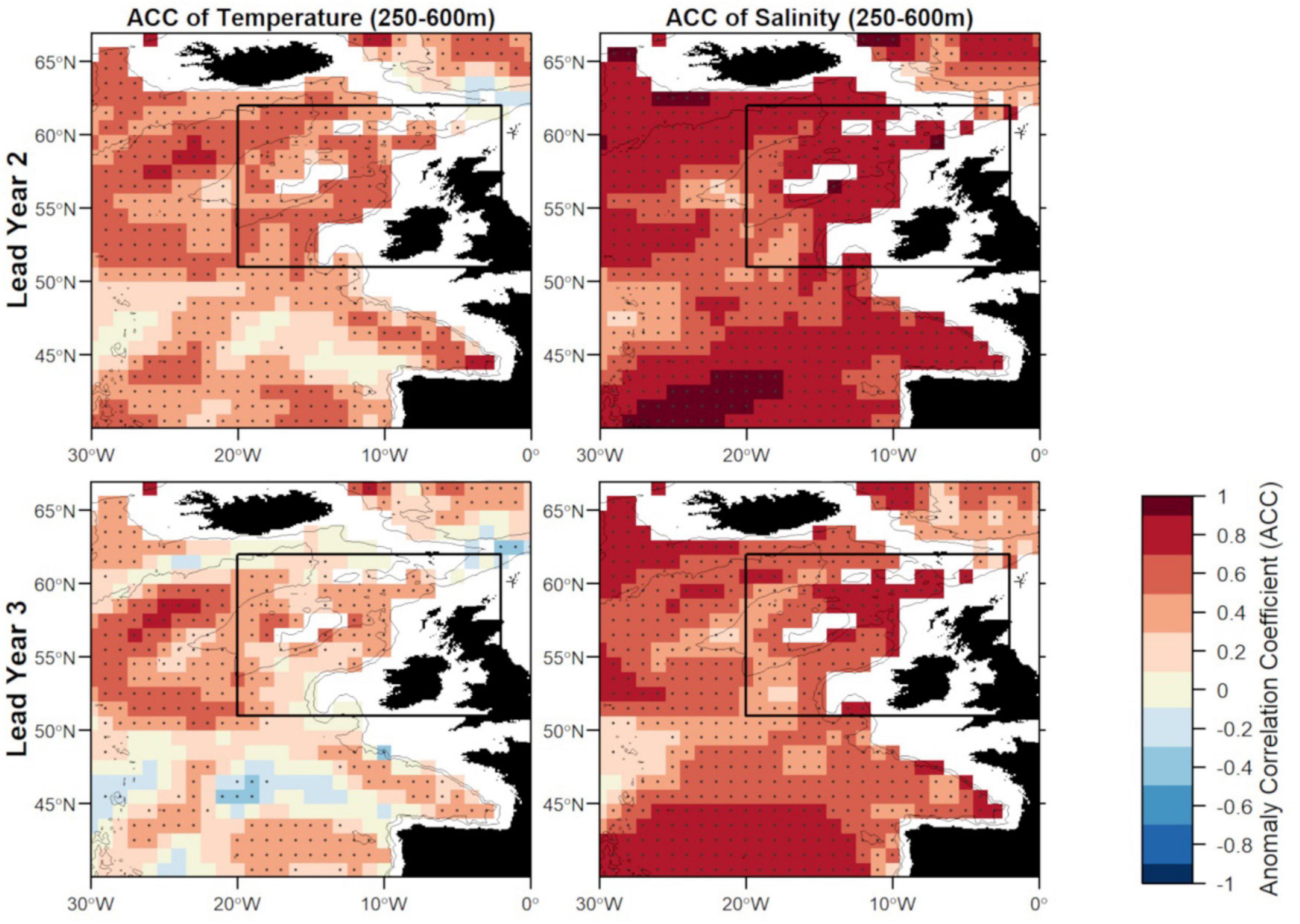
Figure 6. Anomaly correlation coefficient (ACC) of temperature (left) and salinity (right) in FMA at lead year 2 (≈16 months) (top) and lead year 3 (≈28 months) (bottom) comparing MPI-ESM-hindcast to MPI-ESM-assim. Dots show significant correlations at the 95% confidence level, calculated from 500 bootstrap samples. The black rectangle delineates the study area: the spawning region of blue whiting; and black lines indicate the 600 and 2,000 m isobath.
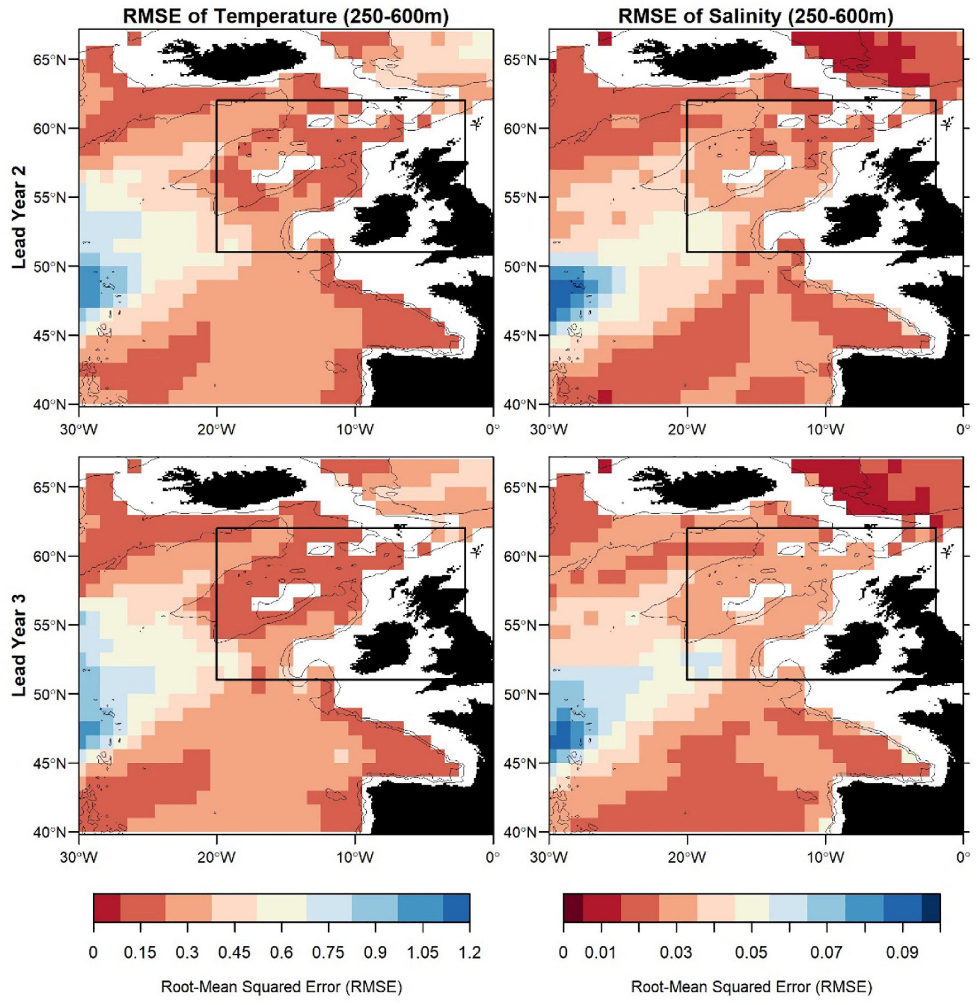
Figure 7. Root-mean squared error (RMSE) of temperature (left) and salinity (right) in FMA at lead year 2 (≈16 months) (top) and lead year 3 (≈28 months) (bottom) comparing MPI-ESM-hindcast to MPI-ESM-assim. The black rectangle delineates the study area: the spawning region of blue whiting.
Zooming into the spawning region of blue whiting, the predictive skill is highest around Rockall Plateau and within Rockall Trough from Porcupine Bank toward the northeast, while predictive skill within the spawning region is lowest in the south-west around 45°N–50°N (Figures 6, 7). In terms of the ACC, MPI-ESM-hindcast of salinity is superior to temperature. However, for lead year 3 a strong decay in predictive skill is seen with regions toward the south–west of the spawning region, where correlations between MPI-ESM-hindcast and MPI-ESM-assim become insignificant for our analysis (Figure 6). Similarly, predictive skill in terms of RMSE is lowest toward the south-west (Figure 7).
Overall, the better hydrodynamic representation of MPI-ESM-assim compared to EN4-analysis together with the high predictive skill of salinity, specifically over longer lead times and in the area around RHP, with MPI-ESM-hindcast, encourage the design of coupled-physical biological forecasts based on MPI-ESM.
The Suitable Spawning Habitat of Blue Whiting defined via SDMs and Salinity
We explore two ways of defining the suitable spawning habitat of blue whiting. In the first approach, SDMs are calibrated using various combinations of temperature and salinity from either MPI-ESM-assim or EN4-analysis (Table 3). For each oceanographic reference product the SDM with the highest predictive performance are SDM_STMPI and SDM_SEN4 (Table 3). These two SDMs are analysed further.
Specifically, for SDMs calibrated with environmental data from MPI-ESM-assim, including salinity and temperature at the spawning depth of blue whiting clearly yields the best performing model in terms of model parsimony with larval CPR data, showing the lowest AIC values and highest explained deviance (SDM_STMPI, Table 3). However, the cross-validated predictive skill of SDM_STMPI is similar to SDM_SEN4, which is the best performing SDM calibrated with EN4-analysis which solely includes salinity as environmental variable (Table 3). Therefore, considering the predictive skill it seems irrelevant whether we use MPI-ESM-assim or EN4-analysis to calibrate the SDMs. For all SDMs the NPV is much larger than the PPV (Table 3), indicating that the SDMs are better in describing the absence of suitable habitat than its presence.
In order to compare output from the SDMs to the suitable salinity for spawning, we convert the likelihood of observing larvae into a binary variable, namely the presence and absence of suitable habitat. The threshold for this conversion is a probability of approximately 0.3 (i.e., for EN4-analysis (MPI-ESM-assim): 0.28 (0.31) in the survey data, and 0.29 (0.34) in the fishery data). Probabilities that exceed (subceed) this threshold translate to presences (absences) of suitable habitat.
For both SDMs, the region defined as suitable for spawning (probability ⪆ 0.3) is centred within the spawning region spanning from the European Continental Shelf onto Rockall Plateau. For SDM_STMPI, however, the suitable spawning habitat extends further west beyond RHP which is not supported by observations (Figures 8A,B). Generally, both SDMs show a more contracted distribution toward the continental shelf in 1991 and a slightly more expanded westward distribution in 2005, however, both fail to reveal the full extent of the observed distributional changes.
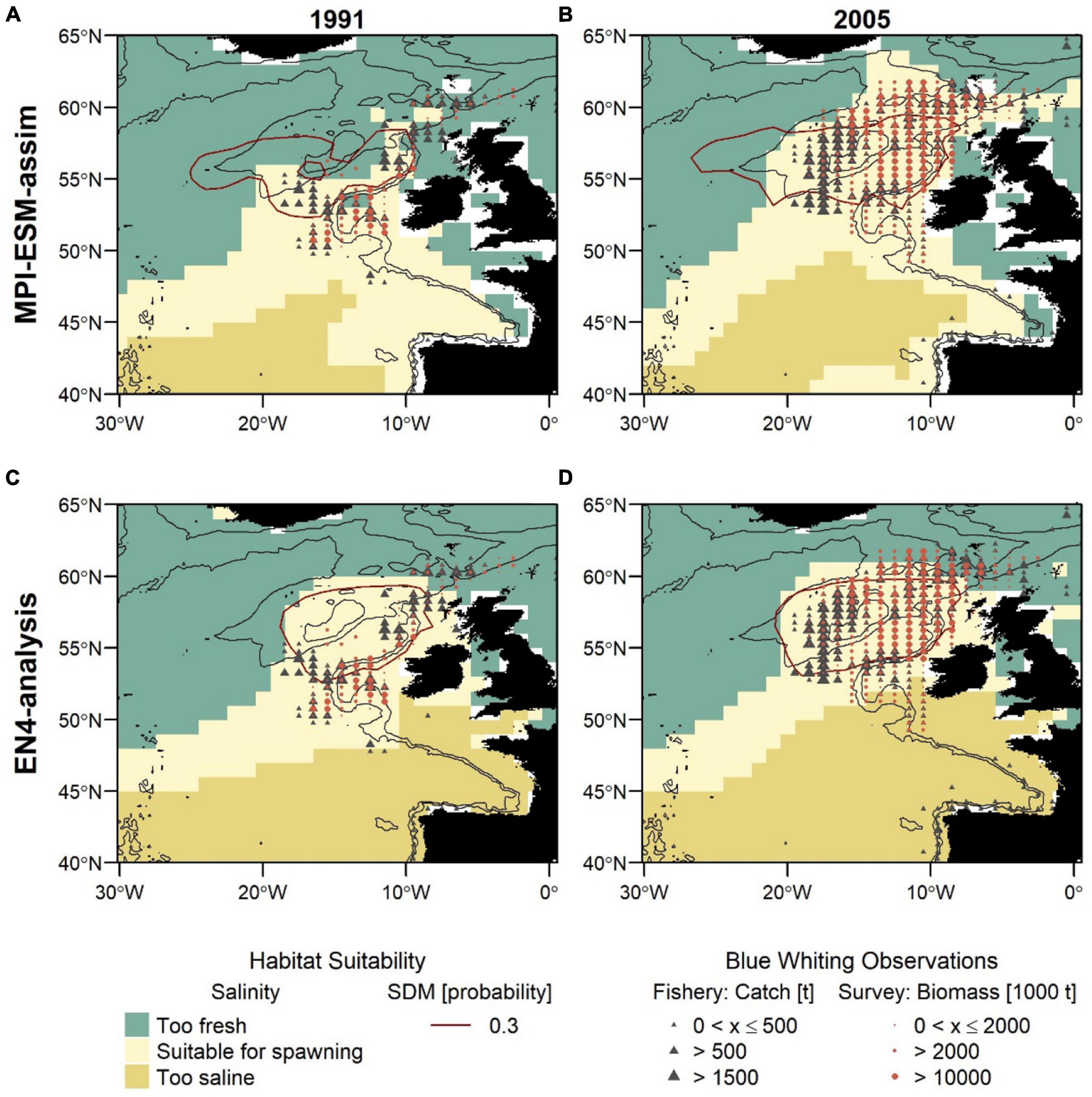
Figure 8. Blue whiting habitat suitability in 1991 (left; A,C) and 2005 (right; B,D) for MPI-ESM-assim (top; A,B) and EN4-analysis (bottom; C,D) compared to observations of adult blue whiting from scientific surveys (IBWSS; red bullet) and fishery catch data (NEAFC; grey triangle) during March and April. Habitat suitability is shown for both the suitable salinity for spawning (background fill) and the probability of observing blue whiting larvae from SDMs (red contour lines; A,B: SDM_STMPI; C,D: SDM_SEN4), where 0.3 resembles the threshold for converting the larval-presence probability into presence and absence of suitable habitat. Bathymetry is indicated by 600 and 2,000 m isobaths.
The second approach uses the suitable salinity for spawning as a proxy for the suitable spawning habitat and there are large differences between the two approaches in the way the suitable habitat is spatially expressed (Figure 8). The suitable salinity for spawning has a considerably larger spatial extent than the suitable habitat based on SDMs and thereby is a better general definition of the potentially suitable habitat that rather overestimates suitable habitat in areas beyond the spawning region of blue whiting. Therefore, the agreement between the suitable salinity for spawning and independent observations is best within the spawning region.
Furthermore, different spatial representations of the marine climate from the two oceanographic reference products affect the spatial distribution of the suitable spawning habitat (Figure 8). The suitable spawning habitat of blue whiting is more affected by the vicinity of bathymetric features, in particular Rockall Plateau, when based on MPI-ESM-assim in comparison to EN4-analysis. The difference between MPI-ESM-assim and EN4-analysis becomes most apparent, however, when comparing the suitable salinity for spawning for two years with contrasting marine climatic regimes. In 1991 the marine climate in the spawning region of blue whiting is characterised by rather cold and fresh conditions (Figure 3) and most blue whiting are observed along the continental shelf from northern Scotland toward Porcupine Bank and south of Rockall Plateau within Rockall Trough (Figures 8A,C). To the contrary in 2005, conditions become more warm and saline in the spawning region (Figure 3) and in response, blue whiting show an expanded spawning distribution that stretches from the continental shelf over RHP with a larger north-westward extent (Figures 8B,D).
While these spatial changes imprint on in the suitable salinity for spawning in MPI-ESM-assim, EN4-analysis fails to resolve changes between 1991 and 2005. In particular in the area around RHP, EN4-analysis shows hardly any difference between the two years (Figures 8C,D), while MPI-ESM-assim reproduces the absence of suitable habitat on Rockall Plateau in 1991 (Figure 8A) and the presence of suitable habitat over most of RHP in 2005 (Figure 8B). Accordingly, the dynamic properties of MPI-ESM-assim and its ability to account for bathymetric constraints might be better suited to reflect the suitable spawning habitat of blue whiting during FMA, in particular in the area of RHP.
Another difference between the two reference products, that is visible for both years is that in MPI-ESM-assim the suitable salinity for spawning extends southward along the continental shelf passing the Spanish and Portuguese coast (Figures 8A,B). This extension is supported by fishery observations (Figures 8A,B).
Within the spawning region, habitat definitions based on the suitable salinity for spawning generally have a higher agreement with independent fishery and survey observations as judged by higher mean values of NPV, HR, and TSS compared to habitat definitions based on SDMs (Table 4). The SDM-based definition is only better in terms of PPV for SDM_SEN4 and the FAR. Both habitat definitions are more useful in describing an absence of suitable habitat within the spawning region (higher NPV) than presence of suitable habitat (lower PPV).
Overall, spatially averaged values of TSS within the spawning region are low (<0.2), however all habitat definitions show greatest agreement with observations from the IBWSS survey in the region around Rockall Plateau and north–east of it (Figure 9). SDM_STMPI shows least agreement with observations (overall TSS = 0) and even displays significantly negative values of TSS in particular around Porcupine Bank (Figure 9A), followed by SDM_SEN4 with an overall TSS of 0.08 (Figure 9B). The suitable spawning habitat in terms of salinity in MPI-ESM-assim shows best agreement with observations from the scientific survey in terms of TSS, with positive values mainly in the north-eastern part of the study region and on RHP (Figure 9C). In contrast to MPI-ESM-assim, differences between the two habitat definitions are smaller for EN4-analysis (Figure 9 and Table 4).
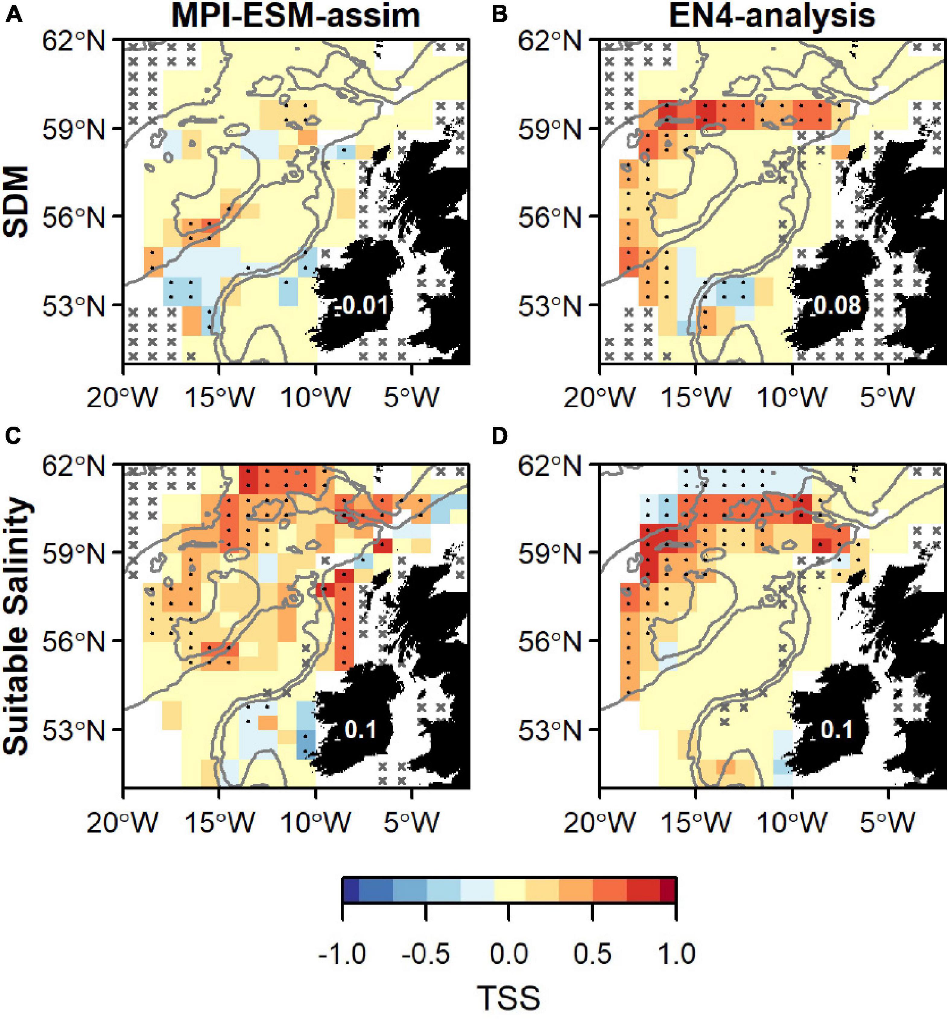
Figure 9. Agreement between the suitable spawning habitat and observations of adult blue whiting from the IBWSS survey in terms of the True Skill Statistics (TSS) during March and April. The suitable spawning habitat is defined through Species Distribution Models (SDM) (top row; A,B) or the suitable salinity for spawning (bottom row; C,D) and based on MPI-ESM-assim (left; A,C) and EN4-analysis (right; B,D). In a and b the best performing SDMs (Table 3) were chosen: SDM_STMPI (A) and SDM_SEN4 (B). Dots show significant correlations at the 95% confidence level and crosses indicate regions where the predictive skill cannot be evaluated confidently due to sparse observational data, both based on a 500-fold bootstrap. Good predictive quality (TSS > 0) is indicated by red colours (where HR > FAR) and the mean TSS within the plotted region (excluding regions with crosses) is noted on Ireland. The grey lines indicate the 600 m and 2,000 m isobath.
Accordingly, the definition of the suitable spawning habitat based on salinity shows better agreement with independent observations than applying the full SDMs. Therefore, we create retrospective forecast of the suitable salinity for spawning and analyse its predictive skill in further detail.
Predictive Skill of the Retrospectively Forecasted Suitable Spawning Habitat Based on Salinity
Generally, retrospective forecasts of the suitable salinity for spawning based on MPI-ESM-hindcast approximately one year ahead have a higher predictive skill than persistence based forecasts (Figure 10). However, overall values of TSS are low with 0.13 when compared to both survey and fishery data and differences to persistence-based forecast are small and in the range of 0.02–0.03 (Figures 10A–C). The predictive skill of all retrospective forecasts is highest on RHP especially west of Rockall Plateau and in the northern part of the spawning region, while low or no predictive skill is found within deeper parts of Rockall Trough and Porcupine Bank (Figures 10A–C). Results are similar when compared to both survey and fishery observations. However, significantly positive TSS values on Rockall Plateau and Porcupine Bank are only found for MPI-ESM-hindcast and MPI-ESM-persist when compared to fishery data (Figures 10A,B). The high predictability of retrospective forecasts on and north-east of RHP, are in line with the high predictability of the marine climate, specifically salinity, found for this region (Figures 6, 7).
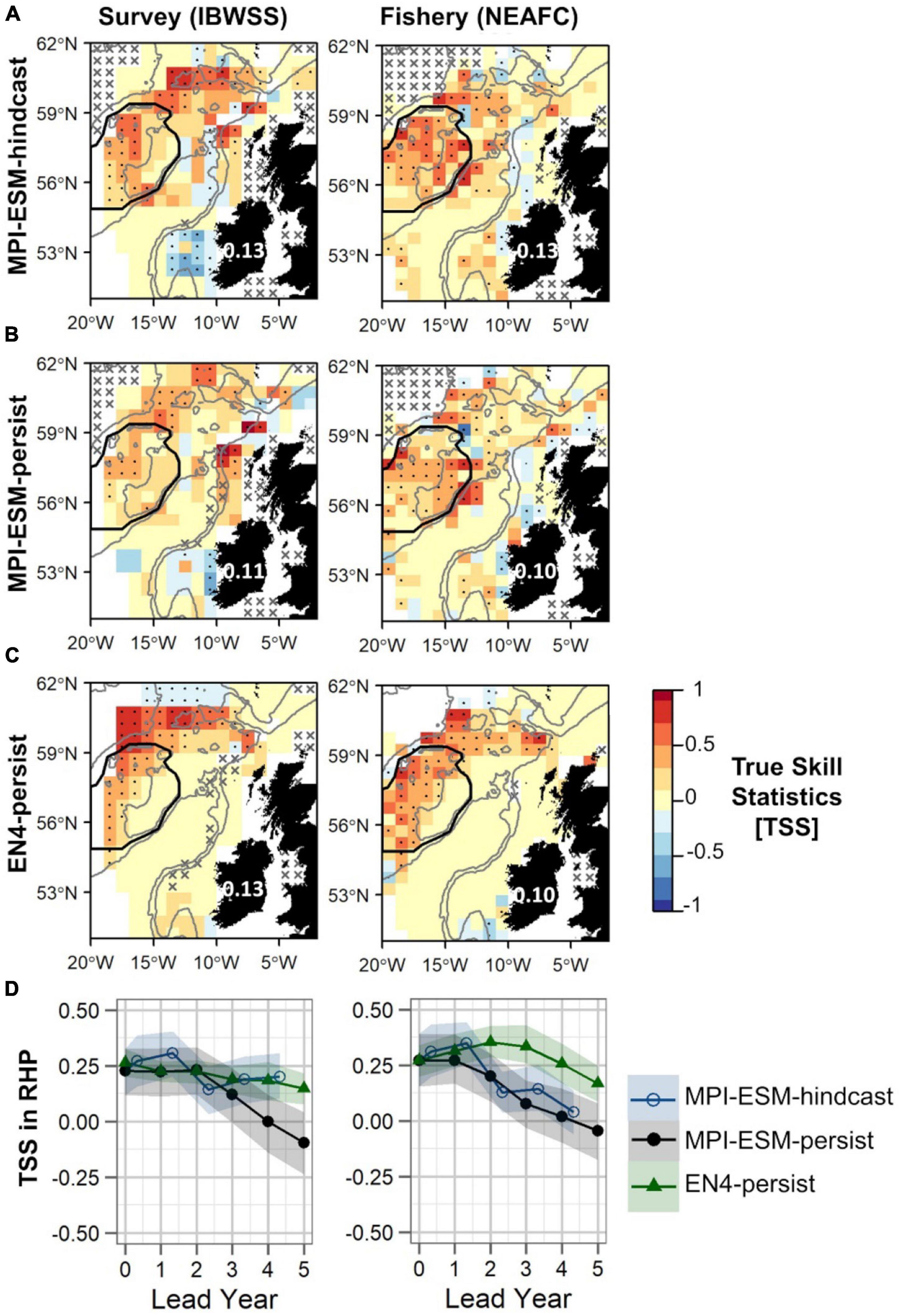
Figure 10. Predictive quality of retrospectively forecasted suitable spawning habitat based on the suitable salinity for spawning with MPI-ESM-hindcast (A), MPI-ESM-persist (B), and EN4-persist (C) in terms of the True Skill Statistics (TSS) for March and April judged against observations of adult blue whiting from surveys (IBWSS) (left) and fishery (NEAFC) (right) approximately one year ahead (A–C); and spatially averaged over Rockall-Hatton Plateau (RHP; region delineated in black in the maps above) for each lead year (D). The last panel (D) shows MPI-ESM-hindcast (blue circle), MPI-ESM-persist (black bullet) and EN4-persist (green triangle) with the shaded areas indicating the spread based on the lower and the upper quartile of a 500-fold bootstrap. Retrospective forecasts are distinctly different when their respective shaded areas do not overlap. Due to the different initialisation dates, panels (A–C) show the hindcast with a lead time of around 16 months and the persistent forecasts with a 12 months lead. In panels (A–C) dots show significant correlations at the 95% confidence level and crosses indicate regions where the predictive skill cannot be evaluated confidently, both based on a 500-fold bootstrap. Good predictive quality (TSS > 0) is indicated by red colours (where HR > FAR) and the mean TSS within the plotted region (excluding regions with crosses) is noted over Ireland. The grey lines indicate the 600 and 2,000 m isobaths.
Within RHP, retrospective forecasts of the suitable salinity for spawning perform similarly for shorter lead times (<2 years) with MPI-ESM-hindcast being slightly but not significantly more skilful than persistence based forecasts (Figure 10D). The forecast horizon at which MPI-ESM-hindcast is more skilful than persistence differs for the two oceanographic data sets and for the two observational data sets of blue whiting. MPI-ESM-hindcast has more skill than MPI-ESM-persist after lead year 3 when assessed by the survey data, however, when compared to the fishery data both show similar skill. EN4-persist shows a similar or higher predictive skill than MPI-ESM-hindcast after lead year 2, as judged by survey and fishery observations, respectively.
Retrospective forecasts of the suitable spawning habitat approximately 1 year in advance show prominent inter-annual variations in predictive skill on RHP, which can roughly be divided into three periods (Figure 11A): From 1985 to 1995, MPI-ESM-hindcast shows the highest skill with values of TSS as high as 0.89 as judged against fishery data while EN4-persist mainly shows no skill. Around the 2000s this reverses when EN4-persist has greater values of TSS than MPI-ESM-hindcast. However, during this time the differences in retrospective forecast skill is high depending on the observational data set chosen and retrospective forecasts based on MPI-ESM-persist and MPI-ESM-hindcast and generally have higher TSS values and hence are more skilful when judged against fishery data in comparison to survey data, indicating a rather large uncertainty in observing blue whiting on RHP. From 2006 onward, forecast skill converges to a range of TSS around 0 to 0.5.
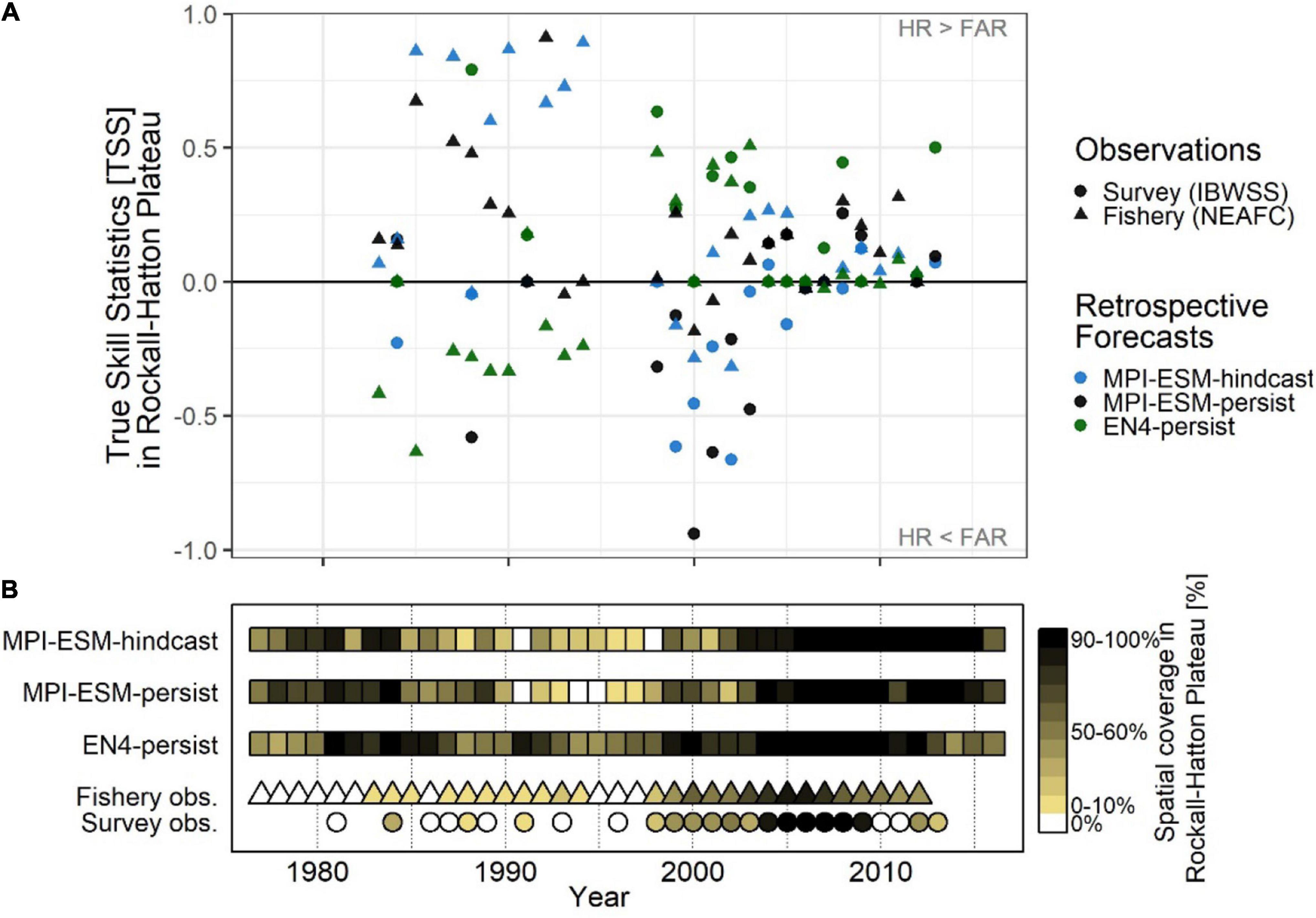
Figure 11. Average inter-annual forecast skill on Rockall-Hatton Plateau (RHP; see Figures 10A–C) in terms of the True Skill Statistics (TSS) (A); and the spatial coverage of suitable spawning habitat in RHP (% of grid cells) (B) based on retrospective forecasts of the suitable salinity for spawning approximately one year ahead with MPI-ESM-hindcast, MPI-ESM-persist and EN4-persist judged against observations of adult blue whiting from surveys (IBWSS; bullet) and fishery (NEAFC; triangle) during March and April. In case observations of blue whiting were absent on RHP [(B): white triangles/bullets = 0%] the TSS is not calculated. Note that observational absences can also indicate that there was no fishing in RHP and shows the absence of IBWSS survey coverage on RHP in the particular year.
These marked changes in the predictive skill over RHP (Figure 11A) coincide with changes in the importance of RHP as a spawning ground (Figure 11B) which in turn are affected by oceanographic variability on the spawning region (Hátún et al., 2009b; Miesner and Payne, 2018). Around 1990 when the marine climate in the spawning region is characterised rather cold and fresh conditions, most spawning takes place along the continental shelf and less on RHP (Hátún et al., 2009a,b; Miesner and Payne, 2018) as shown for 1991 (Figures 8A,C). The importance of RHP as a spawning ground stays low until 1998 with less (or equal) than 30% of blue whiting being observed or caught on RHP (Figure 11B). Likewise, MPI-ESM-persist and particularly MPI-ESM-hindcast show only small fractions of RHP with suitable spawning habitat around 1990 (Figure 11B), resulting in unprecedentedly high forecast skill with values of TSS of 0.85 (Figure 11A). In contrast, EN4-persist constantly shows suitable habitat in more than 30% of RHP. This inability of EN4-analysis to show the absence of suitable spawning habitat over RHP leads to the low predictive skill of EN4-persist until around 1998 (Figure 11).
After 1998 both temperature and salinity increase in the spawning region (Figure 3) which is associated with a north- and westward expansion so the spawning distribution (Hátún et al., 2009a,b; Miesner and Payne, 2018) and blue whiting are observed over a larger area of RHP (Figure 11B). In line with observations from the Ellet Line (Holliday et al., 2015), EN4-analysis shows an increase in temperature and salinity above the climatological average from around 2000–2009 (Figure 3). MPI-ESM-assim, however shows negative anomalies, particularly in salinity around 2000 (Figure 3). Accordingly, MPI-ESM-hindcast and MPI-ESM-persist both underestimate the suitability of the spawning habitat (Figure 11B) resulting in the absence of skill over RHP around 2000 (Figure 11A). In congruence with the period of high temperature and salinity around 2005, which is found in both EN4-analysis and MPI-ESM-assim (Figure 3), also the spatial coverage of blue whiting over RHP peaks and blue whiting are observed over most (if not all) of RHP (Figure 11B). Since all retrospective forecasts also show suitable spawning habitat on RHP (Figure 11B), forecasts skill converges with mainly positive TSS values, in particular for persistence based forecasts (Figure 11A).
In summary, a clear advantage of creating forecasts of the suitable spawning habitat of blue whiting with MPI-ESM compared to EN4-analysis, is the ability of MPI-ESM to differentiate between the presence and absence of suitable spawning habitat over RHP. In particular, MPI-ESM-hindcast skilfully forecasts distributional changes over RHP around a year in advance.
Discussion
We find a higher predictability of salinity compared to temperature within the spatio-temporal domain relevant for spawning blue whiting. Few studies explicitly compare the predictability of salinity and temperature, as presented in this study. One exception is a perfect model experiment that indicated that sea surface salinity is potentially more predictable at inter-annual timescales than sea surface temperature for most oceanic regions of the mid to high latitudes, including the Northeast Atlantic (Koenigk and Mikolajewicz, 2009). In another study, sea surface salinity within the SPG region showed a higher potential predictability compared to both sea surface temperature and upper 300 m heat content with ACC of salinity as high as 0.8 for lead year 2–5 (Mignot et al., 2016), similar to the skill of MPI-ESM-hindcast versus MPI-ESM-assim in our study (Figure 4B). While the mean RMSE for lead year 2–5 of around 0.5 for temperature and 0.05 for salinity (Mignot et al., 2016) is slightly higher than our results indicate (Figures 4C,D, 5C,D).
The marine climate in the spawning region of blue whiting is influenced by the low-frequency dynamics of the SPG that contributes to recurrent periods of relatively high or relatively low salinity spanning over 5–10 years (Holliday et al., 2000; Koul et al., 2019). The salinity signal from the SPG is passively advected with the general ocean circulation toward the North East Atlantic (Mauritzen et al., 2006) and thereby into the spawning region of blue whiting. As such, salinity acts as an indicator for circulation changes in the subpolar North Atlantic (Mauritzen et al., 2006) and the low-frequency dynamics of the SPG that acts on (multi-) decadal timescales (Koul et al., 2019) likely contributes to the high predictability of salinity in spawning region of blue whiting. Specifically, the upper ocean at RHP and the north-eastern Rockall Trough in the vicinity of the continental slope generally show lower oceanographic variability (Holliday et al., 2015) with recurrent and prolonged periods of anomalously high/low salinity (Holliday et al., 2000; Koul et al., 2019). Therefore, predictions of the marine climate and the suitable habitat with MPI-ESM-hindcast show particularly high levels of predictive skill around RHP and in the north-eastern spawning region.
To the contrary, variations in the strength of the SPG affect the position and flow trajectory of the North Atlantic Current and thereby introduce oceanographic variability in the area of Rockall Trough (Holliday et al., 2000; Hátún et al., 2009a; Koul et al., 2019). Rockall Trough is one of the main pathways of the North Atlantic Current, in particular, when the SPG is strong, while the current branches off west of Rockall Plateau, when the SPG is weak (Hátún et al., 2005; Holliday et al., 2020). This oceanographic variability affects the predictability of the marine climate in the Eastern North Atlantic resulting in particularly low predictive skill at the entrance of Rockall Trough in the south-western area of the spawning region.
One key result from this study is that differences in the spatial representation of the marine climate affect the spatial expression of the suitable spawning habitat. Differences in the spatial representation of the marine climate arise from the different methods that are used in EN4-analysis and MPI-ESM-assim to distribute information of observed oceanic temperature and salinity profiles over the study region in time and space. As a dynamic ocean model, MPI-ESM-assim inherently accounts for dynamics and bathymetric features by distributing oceanic properties such as temperature and salinity dynamically consistent around ridges and seamounts such as Rockall Plateau and through channels like Rockall Trough (Figures 1A,B). In contrast, in EN4-analysis observational gaps are filled by means of statistics and not physics. The objective interpolation used in EN4-analysis statistically interpolates between observed profiles and is therefore less capable of representing hydrodynamics, resulting in rather smooth contours of temperature and salinity, disconnected from bathymetry.
The more differentiated representation of the marine climate around bathymetric features in MPI-ESM-assim, results in a superior ability of MPI-ESM-persist and MPI-ESM-hindcast to predict the absence of suitable habitat on RHP. Skilfully forecasting distributional changes of the suitable spawning habitat on RHP could be particular value to the scientific monitoring and management of the stock. Distributional changes are most pronounced on RHP (Hátún et al., 2009b; Miesner and Payne, 2018). Moreover, sampling on RHP is challenging. In particular, the great distance to ports and recurrent periods of bad weather have resulted in insufficient survey coverage on RHP in some years (e.g., 2010) which can lead to an underestimation of the stock’s biomass (ICES, 2010). Therefore, the high inter-annual predictive skill of the marine climate and the suitable spawning habitat around RHP with MPI-ESM with marks a success.
A major challenge that is common to all ecological forecasts that aim at forecasting the spatial distribution of living organisms, is the way habitat is related to the distribution of a species (Payne et al., 2017). Here, the suitable spawning habitat of blue whiting delineates environmental conditions that are suitable for spawning (i.e., in terms of salinity). However, just because a region is suitable for spawning does not necessarily mean that the location is occupied by the fish and spawning takes place. Due to non-resolved processes such as migration dynamics, density dependent effects on distribution or other biotic interactions such competition and predation, not the entire suitable habitat is necessarily occupied by the species (Guisan and Zimmermann, 2000; Colwell and Rangel, 2009; Elith and Leathwick, 2009). Therefore, the actual distribution might be smaller than their potentially suitable habitat, which is clearly seen for the suitable salinity for spawning (Figure 8). While the SDMs delineate the core spawning region west of the British Isles, which is recognised to be the main spawning region of blue whiting (Bailey, 1982; ICES, 2019), they underestimate the spatial (i.e., latitudinal) extent of the spawning distribution. Possible reasons are that the SDMs are constrained by geographic and spatio-temporal parameters and the choice of the threshold for converting probabilities into presences of suitable habitat.
Since habitat models are superior in predicting absences compared to presences, as seen for both approaches applied in this study (Tables 3, 4), the skill of forecasting species distributions is asymmetric (Payne et al., 2021). Consequently, retrospective forecasts of the suitable spawning habitat (e.g., on RHP) with MPI-ESM-hindcast, have higher skill in predicting the absence of suitable habitat (i.e., no spawning on RHP) than their presence.
Nevertheless, instantaneous observations of freely moving animals, like fish, only provide a snapshot of their distribution. We cannot be certain whether the observed adult blue whiting were actively spawning or migrating. Additionally, observations might not cover the entire spawning distribution, e.g., fishermen focus on the most profitable regions with highest fish aggregations while smaller aggregations might be left untouched. Therefore, observations of fish carry uncertainties that affect the assessment biological forecast skill. In particular, our analysis of inter-annual biological forecasts reveals at times massive differences in skill when judged by either fishery or survey data. This highlights the need to consider multiple biological observational data sets for validating coupled physical-biological forecasts.
We define the suitable spawning habitat of blue whiting based on SDMs in a generalised additive modelling framework (Miesner and Payne, 2018). There is, however, a multitude of other modelling options. We cannot rule out that another statistical SDM approach, for example, based on machine learning such as random forest (Breiman, 2001) which is designed for generating predictions (Elith and Leathwick, 2009) might have resulted in a better performance of SDM-based predictions. Additionally applying an ensemble of different modelling techniques would enable accounting for uncertainty in defining the suitable habitat (Araújo and New, 2007).
Salinity seems to be a good proxy for the spawning distribution of blue whiting within its spawning region because it shows good agreement with independent observations (Miesner and Payne, 2018). Salinity can have a direct effect on fish, in particular on early life stages, by affecting their osmoregulation (Varsamos et al., 2005) or egg (Sundby and Kristiansen, 2015) and larval buoyancy as shown for blue whiting (Ådlandsvik et al., 2001). Compared to temperature, however, salinity has a less direct effect on most marine organisms (Rijnsdorp et al., 2009). Therefore, salinity is most likely a proxy for other processes that affect the spawning distribution of blue whiting more directly. Most notably, temperature and salinity are often correlated and form central water mass characteristics. Since each water mass possesses characteristic hydrographic and biogeochemical properties, it functions as distinct habitat for marine organisms. Saline waters of subtropical origin provide a higher abundance of warm-water zooplankton species which are smaller (Hátún et al., 2009a) and thus more favourable prey items of blue whiting larvae (Bailey, 1982) than larger zooplankton species that occupy fresher subpolar waters (Hátún et al., 2009a). Consequently, the suitable salinity for spawning might resemble subtropical water masses with good feeding conditions for blue whiting larvae. The feature of salinity to act as a passive tracer, unmodulated by atmospheric processes, might contribute to the more prominent role of salinity, as opposed to temperature, for defining the suitable spawning habitat of blue whiting.
Due to the imminent importance of salinity as water mass characteristic, it might also be promising to consider salinity for characterising the species–environment relationship of other marine organisms and for creating coupled physical-biological forecasts. The importance of salinity for anticipating distributional changes has also been shown for a range of pelagic species along the US Northeast Shelf (McHenry et al., 2019). The study emphasised that bottom salinity was generally more important in explaining range shifts than temperature, and that projections based solely on temperature masked the species’ climate vulnerability (McHenry et al., 2019). This highlights the prominence of salinity as independent variable in statistical models that predict spatial changes of marine organisms. In agreement, we also find that salinity prediction skill bears a great potential for creating novel coupled physical–biological forecasts.
In regions where local predictability of the marine climate is low, a potential for creating coupled physical–biological forecasts might lie in lagged correlations from regions of high predictability, such as the SPG region. Changes in the SPG affect the relative share of water masses in the Eastern North Atlantic and result in large bio-geographical shifts of blue whiting and a variety of other marine organisms ranging from phyto- and zooplankton, to whales and seabirds (Drinkwater et al., 2003; Hátún et al., 2009a). Additionally, SPG-driven changes of temperature and salinity travel downstream into the North Sea (Núñez-Riboni and Akimova, 2017; Koul et al., 2019) and Barents Sea, and thereby affect the abundance and productivity of some local fish species and introduce predictability via adjective delays (Akimova et al., 2016; Koul et al., 2021). Since retrospective forecasts of the marine climate with MPI-ESM-hindcast in the SPG region show significant skill (Brune et al., 2018; Brune and Baehr, 2020), and Post et al. (2021) found a lagged response between the marine climate south-west of Iceland and the abundance of blue whiting and other boreal fish species in Greenlandic waters, we envision a great potential for developing coupled physical–biological forecasts of fish abundance and distribution based on MPI-ESM in the North Atlantic and its adjacent seas (Koul et al., 2021).
Conclusion
Using blue whiting as a case study, we show that MPI-ESM-hindcast skilfully predicts the marine climate, specifically salinity, in the North East Atlantic several years ahead, which translates to predictability of distributional shifts in the species’ suitable spawning habitat a year in advance. We find that the suitable salinity for spawning proves to be a better proxy for the suitable spawning habitat than applying a SDM. While the definition of the suitable habitat is species specific and requires careful consideration, many aspects from this study can be generalised and are also applicable to other species. Hence, ESMs bear great potentials for forecasting fish distributions in the North East Atlantic.
One of the main advantages in delineating and forecasting the suitable habitat with MPI-ESM is the ESM’s representation of hydrographic processes, which is superior to the statistical product EN4-analysis for the conducted analysis. The dynamic consistency and ability of an ESM to consider hydrodynamics can therefore offer advantages over a solely statistical oceanographic data product, specifically for coupled physical–biological forecasts in regions with distinct bathymetry, e.g., over seamounts, plateaus or shelfs, which typically depict preferred habitat features for many marine species, as seen for blue whiting. Since skilful biological forecasts at inter-annual time scales, as presented in this study, are beyond the prediction horizon of the first generation of biological forecast products (Payne et al., 2017), they present an innovation of marine biological forecasts.
Another insight from this study is the higher predictive skill of deep-water salinity compared to temperature and its impending importance as water mass and habitat characteristic in the North East Atlantic. For many commercially important fish species in the North Atlantic a wealth of observational records exist and environmental drivers for distributional changes are known (Trenkel et al., 2014; and references therein). This could offer the possibility to delineate the species’ suitable habitat by combining existing observations of the species in combination with skilful observational oceanographic data sets. Moreover, including salinity in coupled physical–biological forecasts could offer a valuable contribution toward predicting distributional shifts of marine living organisms and for creating novel marine ecological forecasts.
Data Availability Statement
Monthly observations of ocean temperature and salinity are available from the Met Office Hadley Centre’s EN4 data set. In this study version EN4.2.1 was used with corrections based on Gouretski and Reseghetti (2010), which can be downloaded at https://www.metoffice.gov.uk/hadobs/en4/download-en4-2-1.html. Temperature and salinity fields for MPI-ESM can be downloaded at https://cera-www.dkrz.de/WDCC/ui/cerasearch/entry?acronym=DKRZ_LTA_1075_ds00008. Bathymetry data from the ETOPO1 Global Relief Model is publicly available at https://www.ngdc.noaa.gov/mgg/global/.
Author Contributions
AM conceived the work, performed the analysis and wrote the manuscript. SB created the MPI-ESM hindcast and assimilation experiments. AM, SB, VK, and PP discussed the results. CS and JB provided guidance on the overall direction of the work. All authors reviewed the manuscript.
Funding
This research is funded through the Earth and Environment Research Programme of the Helmholtz Association Germany and is a contribution to the Subtopic “Coastal System Sustainability against the Backdrop of Natural and Anthropogenic Drivers” of Topic 4 “Coastal Transition Zones under Natural and Human Pressure” of the PoF IV research program Earth and Environment “Changing Earth-Sustaining our Future.” Moreover, the study is funded by the Deutsche Forschungsgemeinschaft (DFG, German Research Foundation) under Germany‘s Excellence Strategy—EXC 2037 “CLICCS—Climate, Climatic Change, and Society”—Project Number: 390683824, contributing to the Center for Earth System Research and Sustainability (CEN) of Universität Hamburg. JB and S.B were supported by Copernicus Climate Change Service, funded by the EU, under contract C3S-330. Analysis of the CPR samples from 1979 to 2005 was funded by the United Kingdom Department of Environment, Fisheries and Rural Affairs (Defra, project MF1101). The funders had no role in study design, data collection and analysis, decision to publish, or preparation of the manuscript.
Conflict of Interest
The authors declare that the research was conducted in the absence of any commercial or financial relationships that could be construed as a potential conflict of interest.
The handling Editor declared a past co-authorship with one of the authors VK.
Publisher’s Note
All claims expressed in this article are solely those of the authors and do not necessarily represent those of their affiliated organizations, or those of the publisher, the editors and the reviewers. Any product that may be evaluated in this article, or claim that may be made by its manufacturer, is not guaranteed or endorsed by the publisher.
Acknowledgments
We wish to thank André Düsterhus for his constructive and helpful comments. Moreover, we wish to thank the German Climate Computing Centre (DKRZ) where the model simulations were performed.
References
Ådlandsvik, B., Coombs, S., Sundby, S., and Temple, G. (2001). Buoyancy and vertical distribution of eggs and larvae of blue whiting (Micromesistius poutassou): observations and modelling. Fish. Res. 50, 59–72. doi: 10.1016/S0165-7836(00)00242-3
Akimova, A., Núñez-Riboni, I., Kempf, A., and Taylor, M. H. (2016). Spatially-resolved influence of temperature and salinity on stock and recruitment variability of commercially important fishes in the north sea. PLoS One 11:e0161917. doi: 10.1371/journal.pone.0161917
Amante, C., and Eakins, B. W. (2009). ETOPO1 1 Arc-Minute Global Relief Model: Procedures, Data Sources and Analysis. NOAA Technical Memorandum NESDIS NGDC. Washington, DC: NOAA, 24. doi: 10.7289/V5C8276M
Anderson, D. R. (2008). Model Based Inference in the Life Sciences: A Primer on Evidence. New York, NY: Springer New York, doi: 10.1007/978-0-387-74075-1
Araújo, M. B., and New, M. (2007). Ensemble forecasting of species distributions. Trends Ecol. Evol. 22, 42–47. doi: 10.1016/j.tree.2006.09.010
Bailey, R. S. (1982). The population biology of blue whiting in the North Atlantic. Adv. Mar. Biol. 19, 257–355. doi: 10.1016/S0065-2881(08)60089-9
Brown, C. D., and Davis, H. T. (2006). Receiver operating characteristics curves and related decision measures: a tutorial. Chemom. Intell. Lab. Syst. 80, 24–38. doi: 10.1016/j.chemolab.2005.05.004
Brune, S., and Baehr, J. (2020). Preserving the coupled atmosphere–ocean feedback in initializations of decadal climate predictions. WIREs Clim. Chang. 11:e637. doi: 10.1002/wcc.637
Brune, S., Düsterhus, A., Pohlmann, H., Müller, W. A., and Baehr, J. (2018). Time dependency of the prediction skill for the North Atlantic subpolar gyre in initialized decadal hindcasts. Clim. Dyn. 51, 1947–1970. doi: 10.1007/s00382-017-3991-4
Brune, S., Nerger, L., and Baehr, J. (2015). Assimilation of oceanic observations in a global coupled Earth system model with the SEIK filter. Ocean Model. 96, 254–264. doi: 10.1016/j.ocemod.2015.09.011
Burnham, K. P., Anderson, D. R., and Huyvaert, K. P. (2011). AIC model selection and multimodel inference in behavioral ecology: some background, observations, and comparisons. Behav. Ecol. Sociobiol. 65, 23–35. doi: 10.1007/s00265-010-1029-6
Colwell, R. K., and Rangel, T. F. (2009). Hutchinson’s duality: the once and future niche. Proc. Natl. Acad. Sci. U.S.A. 106(Suppl. 2), 19651–19658. doi: 10.1073/pnas.0901650106
Coombs, S. H., Pipe, R. K., and Mitchell, C. E. (1981). The vertical distribution of eggs and larvae of blue whiting (Micromesistius poutassou) and Mackerel (Scomber scombrus) in the Eastern North Atlantic and North Sea. Rapp. Proc. Verb. Cons. Int. Explor. Mer 178, 188–195.
Dee, D. P., Uppala, S. M., Simmons, A. J., Berrisford, P., Poli, P., Kobayashi, S., et al. (2011). The ERA-Interim reanalysis: configuration and performance of the data assimilation system. Q. J. R. Meteorol. Soc. 137, 553–597. doi: 10.1002/qj.828
Drinkwater, K. F., Belgrano, A., Borja, A., Conversi, A., Edwards, M., Greene, C. H., et al. (2003). “The response of marine ecosystems to climate variability associated with the North Atlantic Oscillation,” in The North Atlantic Oscillation: Climatic Significance and Environmental Impact, eds J. W. Hurrell, Y. Kushnir, G. Ottersen, and M. Visbeck (Washington, DC: American Geophysical Union), 211–234. doi: 10.1029/134GM10
Elith, J., and Leathwick, J. R. (2009). Species distribution models: ecological explanation and prediction across space and time. Annu. Rev. Ecol. Evol. Syst. 40, 415–436. doi: 10.1146/annurev.ecolsys.l
Eveson, J. P., Hobday, A. J., Hartog, J. R., Spillman, C. M., and Rough, K. M. (2015). Seasonal forecasting of tuna habitat in the Great Australian Bight. Fish. Res. 170, 39–49. doi: 10.1016/j.fishres.2015.05.008
Freeman, E. A., and Moisen, G. G. (2008). A comparison of the performance of threshold criteria for binary classification in terms of predicted prevalence and kappa. Ecol. Modell. 217, 48–58. doi: 10.1016/j.ecolmodel.2008.05.015
Frölicher, T. L., Ramseyer, L., Raible, C. C., Rodgers, K. B., and Dunne, J. (2020). Potential predictability of marine ecosystem drivers. Biogeosciences 17, 2061–2083. doi: 10.5194/bg-17-2061-2020
Giorgetta, M. A., Jungclaus, J., Reick, C. H., Legutke, S., Bader, J., Böttinger, M., et al. (2013). Climate and carbon cycle changes from 1850 to 2100 in MPI-ESM simulations for the coupled model intercomparison project phase 5. J. Adv. Model. Earth Syst. 5, 572–597. doi: 10.1002/jame.20038
Good, S. A., Martin, M. J., and Rayner, N. A. (2013). EN4: quality controlled ocean temperature and salinity profiles and monthly objective analyses with uncertainty estimates. J. Geophys. Res. Ocean. 118, 6704–6716. doi: 10.1002/2013JC009067
Gouretski, V., and Reseghetti, F. (2010). On depth and temperature biases in bathythermograph data: development of a new correction scheme based on analysis of a global ocean database. Deep Res. Part I 57, 812–833. doi: 10.1016/j.dsr.2010.03.011
Guisan, A., and Zimmermann, N. E. (2000). Predictive habitat distribution models in ecology. Ecol. Modell. 135, 147–186. doi: 10.1016/S0304-3800(00)00354-9
Hátún, H., Payne, M. R., Beaugrand, G., Reid, P. C., Sandø, A. B., Drange, H., et al. (2009a). Large bio-geographical shifts in the north-eastern Atlantic Ocean: from the subpolar gyre, via plankton, to blue whiting and pilot whales. Prog. Oceanogr. 80, 149–162. doi: 10.1016/j.pocean.2009.03.001
Hátún, H., Payne, M. R., and Jacobsen, J. A. (2009b). The North Atlantic subpolar gyre regulates the spawning distribution of blue whiting (Micromesistius poutassou). Can. J. Fish. Aquat. Sci. 66, 759–770. doi: 10.1139/F09-037
Hátún, H., Sandø, A. B., Drange, H., Hansen, B., and Valdimarsson, H. (2005). Influence of the Atlantic Subpolar Gyre on the thermohaline circulation. Scienc 309, 1841–1844. doi: 10.1126/science.1114777
Heino, M., Engelhard, G. H., and Godø, O. R. (2008). Migrations and hydrography determine the abundance fluctuations of blue whiting (Micromesistius poutassou) in the Barents Sea. Fish. Oceanogr. 17, 153–163. doi: 10.1111/j.1365-2419.2008.00472.x
Hillgruber, N., and Kloppmann, M. (1999). Distribution and feeding of blue whiting Micromesistius poutassou larvae in relation to different water masses in the Porcupine Bank area, west of Ireland. Mar. Ecol. Prog. Ser. 187, 213–225. doi: 10.3354/meps187213
Hillgruber, N., and Kloppmann, M. (2000). Vertical distribution and feeding of larval blue whiting in turbulent waters above Porcupine Bank. J. Fish Biol. 57, 1290–1311. doi: 10.1111/j.1095-8649.2000.tb00488.x
Hobday, A. J., and Hartmann, K. (2006). Near real-time spatial management based on habitat predictions for a longline bycatch species. Fish. Manag. Ecol. 13, 365–380. doi: 10.1111/j.1365-2400.2006.00515.x
Hobday, A. J., Hartog, J. R., Spillman, C. M., and Alves, O. (2011). Seasonal forecasting of tuna habitat for dynamic spatial management. Can. J. Fish. Aquat. Sci. 68, 898–911. doi: 10.1139/f2011-031
Hobday, A. J., Spillman, C. M., Paige Eveson, J., and Hartog, J. R. (2016). Seasonal forecasting for decision support in marine fisheries and aquaculture. Fish. Oceanogr. 25, 45–56. doi: 10.1111/fog.12083
Holliday, N. P., Bersch, M., Berx, B., Chafik, L., Cunningham, S., Florindo-López, C., et al. (2020). Ocean circulation causes the largest freshening event for 120 years in eastern subpolar North Atlantic. Nat. Commun. 11:585. doi: 10.1038/s41467-020-14474-y
Holliday, N. P., Cunningham, S. A., Johnson, C., Gary, S. F., Griffiths, C., Read, J. F., et al. (2015). Multidecadal variability of potential temperature, salinity, and transport in the eastern subpolar North Atlantic. J. Geophys. Res. Ocean. 120, 5945–5967. doi: 10.1002/2015JC010762
Holliday, N. P., Pollard, R. T., Read, J. F., and Leach, H. (2000). Water mass properties and fluxes in the Rockall Trough, 1975-1998. Deep Res. Part I Oceanogr. Res. Pap. 47, 1303–1332. doi: 10.1016/S0967-0637(99)00109-0
ICES (2010). Advice October 2010. Widely Distributed and Migratory Stocks Blue Whiting in Subareas I – IX, XII, and XIV. Available online at: https://www.ices.dk/sites/pub/PublicationReports/Advice/2010/2010/whb-comb.pdf (accessed September 9, 2021).
ICES (2015). Manual for International Pelagic Surveys (IPS). Series of ICES Survey Protocols SISP 9. Version 1.00. Working Group of International Pelagic Surveys. Copenhagen: ICES. doi: 10.17895/ices.pub/7582
ICES (2016). Stock Annex for Blue Whiting (Subareas I-IX, XI I and XIV). Working Group for Widely Distributed Stocks. 1–36. Available online at: https://www.ices.dk/sites/pub/PublicationReports/StockAnnexes/2016/whb-comb_SA.pdf (accessed September 9, 2021).
ICES (2018). Interim Report of the Working Group on Seasonal to Decadal Prediction of Marine Ecosystems (WGS2D). Copenhagen: ICES, 42.
ICES (2019). Stock Annex: Blue Whiting (Micromesistius poutassou) in Subareas 1-9, 12, and 14 (Northeast Atlantic and Adjacent Waters). Available online at: https://www.ices.dk/sites/pub/PublicationReports/StockAnnexes/2019/whb.27.1-91214_SA.pdf (accessed September 9, 2021).
Johnson, D. E., Barrio Froján, C., Neat, F., Van Oevelen, D., Stirling, D., Gubbins, M. J., et al. (2019). Rockall and Hatton: resolving a super wicked marine governance problem in the high seas of the Northeast Atlantic Ocean. Front. Mar. Sci. 6:69. doi: 10.3389/fmars.2019.00069
Jolliffe, I. T., and Stephenson, D. B. (2012). Forecast Verification: A Practitioner’s Guide in Atmospheric Science, 2nd Edn, eds I. T. Jolliffe and D. B. Stephenson (Chichester: Wiley-Blackwell).
Jungclaus, J. H., Fischer, N., Haak, H., Lohmann, K., Marotzke, J., Matei, D., et al. (2013). Characteristics of the ocean simulations in the Max Planck Institute Ocean Model (MPIOM) the ocean component of the MPI-Earth system model. J. Adv. Model. Earth Syst. 5, 422–446. doi: 10.1002/jame.20023
Kaplan, I. C., Williams, G. D., Bond, N. A., Hermann, A. J., and Siedlecki, S. A. (2016). Cloudy with a chance of sardines: forecasting sardine distributions using regional climate models. Fish. Oceanogr. 25, 15–27. doi: 10.1111/fog.12131
Koenigk, T., and Mikolajewicz, U. (2009). Seasonal to interannual climate predictability in mid and high northern latitudes in a global coupled model. Clim. Dyn. 32, 783–798. doi: 10.1007/s00382-008-0419-1
Koul, V., Schrum, C., Düsterhus, A., and Baehr, J. (2019). Atlantic Inflow to the North Sea modulated by the Subpolar Gyre in a Historical simulation With MPI-ESM. J. Geophys. Res. Ocean. 124, 1807–1826. doi: 10.1029/2018JC014738
Koul, V., Sguotti, C., Årthun, M., Brune, S., Düsterhus, A., Bogstad, B., et al. (2021). Skilful prediction of cod stocks in the North and Barents Sea a decade in advance. Commun. Earth Environ. 2:140. doi: 10.1038/s43247-021-00207-6
Lehodey, P., Senina, I., Wibawa, T. A., Titaud, O., Calmettes, B., Conchon, A., et al. (2018). Operational modelling of bigeye tuna (Thunnus obesus) spatial dynamics in the Indonesian region. Mar. Pollut. Bull. 131, 19–32. doi: 10.1016/j.marpolbul.2017.08.020
Liu, C., White, M., and Newell, G. (2011). Measuring and comparing the accuracy of species distribution models with presence-absence data. Ecography (Cop.) 34, 232–243. doi: 10.1111/j.1600-0587.2010.06354.x
Malick, M. J., Siedlecki, S. A., Norton, E. L., Kaplan, I. C., Haltuch, M. A., Hunsicker, M. E., et al. (2020). Environmentally driven seasonal forecasts of Pacific Hake distribution. Front. Mar. Sci. 7:578490. doi: 10.3389/fmars.2020.578490
Matei, D., Pohlmann, H., Jungclaus, J. H., Müller, W., Haak, H., and Marotzke, J. (2012). Two Tales of initializing decadal climate prediction experiments with the ECHAM5/MPI-OM Model. J. Clim. 25, 8502–8523. doi: 10.1175/JCLI-D-11-00633.1
Mauritzen, C., Hjøllo, S. S., and Sandø, A. B. (2006). Passive tracers and active dynamics: a model study of hydrography and circulation in the northern North Atlantic. J. Geophys. Res. 111:C08014. doi: 10.1029/2005JC003252
McHenry, J., Welch, H., Lester, S. E., and Saba, V. (2019). Projecting marine species range shifts from only temperature can mask climate vulnerability. Glob. Chang. Biol. 25, 4208–4221. doi: 10.1111/gcb.14828
Miesner, A. K., and Payne, M. R. (2018). Oceanographic variability shapes the spawning distribution of blue whiting (Micromesistius poutassou). Fish. Oceanogr. 27, 623–638. doi: 10.1111/fog.12382
Mignot, J., García-Serrano, J., Swingedouw, D., Germe, A., Nguyen, S., Ortega, P., et al. (2016). Decadal prediction skill in the ocean with surface nudging in the IPSL-CM5A-LR climate model. Clim. Dyn. 47, 1225–1246. doi: 10.1007/s00382-015-2898-1
NEAFC (2013). Report from the NEAFC Working Group on Collating Information on the Distribution of All Life Stages of Blue Whiting in the North-East Atlantic and the Distribution of Catches from the Stock, London, 26 – 28 November 2013. London: NEAFC.
Núñez-Riboni, I., and Akimova, A. (2017). Quantifying the impact of the major driving mechanisms of inter-annual variability of salinity in the North Sea. Prog. Oceanogr. 154, 25–37. doi: 10.1016/j.pocean.2017.04.004
Payne, M. R. (2021). Blue Whiting Spawning Habitat Forecast. ICES WGS2D Forecast Sheet 01-20210118. 1–6. Available online at: https://fishforecasts.dtu.dk/forecasts/blue-whiting-spawning-habitat (accessed October 21, 2021).
Payne, M. R., and Lehodey, P. (2019). “Review of the use of ocean data in European fishery management and monitoring applications,” in Copernicus Marine Service Ocean State Report. Issue 3. Journal of Operational Oceanography. 12:Sup1, eds K. von Schuckmann and P.-Y. Le Traon (London: Taylor & Francis), 48–52. doi: 10.1080/1755876X.2019.1633075
Payne, M. R., Hobday, A. J., MacKenzie, B. R., Tommasi, D., Dempsey, D. P., Fässler, S. M. M., et al. (2017). Lessons from the first generation of marine ecological forecast products. Front. Mar. Sci. 4:289. doi: 10.3389/fmars.2017.00289
Payne, M. R., Miesner, A. K., Keenlyside, N., Yang, S., and Yeager, S. G. (2021). Skilful decadal-scale distribution shifts prediction of fish habitat. bioRxiv [Preprint] 1–23. doi: 10.1101/2021.07.07.451446
Pointin, F., and Payne, M. R. (2014). A Resolution to the blue whiting (Micromesistius poutassou) population paradox? PLoS One 9:e106237. doi: 10.1371/journal.pone.0106237
Polkova, I., Brune, S., Kadow, C., Romanova, V., Gollan, G., Baehr, J., et al. (2019). Initialization and ensemble generation for decadal climate predictions: a comparison of different methods. J. Adv. Model. Earth Syst. 11, 149–172. doi: 10.1029/2018MS001439
Post, S., Fock, H. O., and Jansen, T. (2019). Blue whiting distribution and migration in Greenland waters. Fish. Res. 212, 123–135. doi: 10.1016/j.fishres.2018.12.007
Post, S., Werner, K. M., Núñez-Riboni, I., Chafik, L., Hátún, H., and Jansen, T. (2021). Subpolar gyre and temperature drive boreal fish abundance in Greenland waters. Fish Fish. 22, 161–174. doi: 10.1111/faf.12512
Reid, P. C., Colebrook, J. M., Matthews, J. B. L., Aiken, J., and Team, C. P. R. (2003). The continuous plankton recorder: concepts and history, from Plankton Indicators to undulating recorders. Prog. Oceanogr. 58, 117–173. doi: 10.1016/j.pocean.2003.08.002
Rijnsdorp, A. D., Peck, M. A., Engelhard, G. H., Möllmann, C., and Pinnegar, J. K. (2009). Resolving the effect of climate change on fish populations. ICES J. Mar. Sci. 66, 1570–1583. doi: 10.1093/icesjms/fsp056
Shaffrey, L. C., Hodson, D., Robson, J., Stevens, D. P., Hawkins, E., Polo, I., et al. (2017). Decadal predictions with the HiGEM high resolution global coupled climate model: description and basic evaluation. Clim. Dyn. 48, 297–311. doi: 10.1007/s00382-016-3075-x
Siedlecki, S. A., Kaplan, I. C., Hermann, A. J., Nguyen, T. T., Bond, N. A., Newton, J. A., et al. (2016). Experiments with seasonal forecasts of ocean conditions for the Northern region of the California current upwelling system. Sci. Rep. 6:27203. doi: 10.1038/srep27203
Sundby, S., and Kristiansen, T. (2015). The principles of buoyancy in marine fish eggs and their vertical distributions across the world oceans. PLoS One 10:e0138821. doi: 10.1371/journal.pone.0138821
Taylor, K. E., Stouffer, R. J., and Meehl, G. A. (2012). An overview of CMIP5 and the experiment design. Bull. Am. Meteorol. Soc. 93, 485–498. doi: 10.1175/BAMS-D-11-00094.1
Tommasi, D., Stock, C. A., Hobday, A. J., Methot, R. R., Kaplan, I. C., Eveson, J. P., et al. (2017a). Managing living marine resources in a dynamic environment: the role of seasonal to decadal climate forecasts. Prog. Oceanogr. 152, 15–49. doi: 10.1016/j.pocean.2016.12.011
Tommasi, D., Stock, C. A., Pegion, K., Vecchi, G. A., Methot, R. D., Alexander, M. A., et al. (2017b). Improved management of small pelagic fisheries through seasonal climate prediction. Ecol. Appl. 27, 378–388. doi: 10.1002/eap.1458
Trenkel, V. M., Huse, G., MacKenzie, B. R., Alvarez, P., Arrizabalaga, H., Castonguay, M., et al. (2014). Comparative ecology of widely distributed pelagic fish species in the North Atlantic: implications for modelling climate and fisheries impacts. Prog. Oceanogr. 129, 219–243. doi: 10.1016/j.pocean.2014.04.030
Uppala, S. M., Kållberg, P. W., Simmons, A. J., Andrae, U., Bechtold, V. D. C., Fiorino, M., et al. (2005). The ERA-40 re-analysis. Q. J. R. Meteorol. Soc. 131, 2961–3012. doi: 10.1256/qj.04.176
Varsamos, S., Nebel, C., and Charmantier, G. (2005). Ontogeny of osmoregulation in postembryonic fish: a review. Comp. Biochem. Physiol. Part A Mol. Integr. Physiol. 141, 401–429. doi: 10.1016/j.cbpb.2005.01.013
Wiens, J. A., Stralberg, D., Jongsomjit, D., Howell, C. A., and Snyder, M. A. (2009). Niches, models, and climate change: assessing the assumptions and uncertainties. Proc. Natl. Acad. Sci. U.S.A. 106, 19729–19736. doi: 10.1073/pnas.0901639106
Wilks, D. S. (2011). Statistical Methods in the Atmospheric Sciences: International Geophysics Series, 3rd Edn, Vol. 100. Amsterdam: Elsevier Inc. doi: 10.1016/B978-0-12-385022-5.00001-4
Yeager, S. G., and Robson, J. I. (2017). Recent progress in understanding and predicting Atlantic Decadal climate variability. Curr. Clim. Chang. Rep. 3, 112–127. doi: 10.1007/s40641-017-0064-z
Keywords: species distribution model, habitat preference, spawning, North Atlantic, climate variability, ecological forecast, prediction, MPI-ESM
Citation: Miesner AK, Brune S, Pieper P, Koul V, Baehr J and Schrum C (2022) Exploring the Potential of Forecasting Fish Distributions in the North East Atlantic With a Dynamic Earth System Model, Exemplified by the Suitable Spawning Habitat of Blue Whiting. Front. Mar. Sci. 8:777427. doi: 10.3389/fmars.2021.777427
Received: 15 September 2021; Accepted: 22 December 2021;
Published: 28 January 2022.
Edited by:
Hjálmar Hátún, Faroe Marine Research Institute (FAMRI), Faroe IslandsReviewed by:
Tommaso Russo, University of Rome Tor Vergata, ItalyGang Hou, Guangdong Ocean University, China
Brian R. MacKenzie, Technical University of Denmark, Denmark
Copyright © 2022 Miesner, Brune, Pieper, Koul, Baehr and Schrum. This is an open-access article distributed under the terms of the Creative Commons Attribution License (CC BY). The use, distribution or reproduction in other forums is permitted, provided the original author(s) and the copyright owner(s) are credited and that the original publication in this journal is cited, in accordance with accepted academic practice. No use, distribution or reproduction is permitted which does not comply with these terms.
*Correspondence: Anna K. Miesner, anna.miesner@hereon.de