Season-Dependent Hedging Policies for Reservoir Operation—A Comparison Study

Abstract

During periods of significant water shortage or when drought is impending, it is customary to implement some kind of water supply reduction measures with a view to prevent the occurrence of severe shortages (vulnerability) in the near future. In the case of operation of a water supply reservoir, this reduction of water supply is affected by hedging schemes or hedging policies. This research work aims to compare the popular hedging policies: (i) linear two-point hedging; (ii) modified two-point hedging; and, (iii) discrete hedging based on time-varying and constant hedging parameters. A parameterization-simulation-optimization (PSO) framework is employed for the selection of the parameters of the compromising hedging policies. The multi-objective evolutionary search-based technique (Non-dominated Sorting based Genetic Algorithm-II) was used to identify the Pareto-optimal front of hedging policies that seek to obtain the trade-off between shortage ratio and vulnerability. The case example used for illustration is the Hemavathy reservoir in Karnataka, India. It is observed that the Pareto-optimal front that was obtained from time-varying hedging policies show significant improvement in reservoir performance when compared to constant hedging policies. The variation in the monthly parameters of the time-variant hedging policies shows a strong correlation with monthly inflows and available water.

1. Introduction

The rule or policy of any reservoir operation involves deciding the amount of releases to be made from the reservoir to meet the specified demands for different purposes based on the “current storage in the reservoir and the expected (likely) inflows to the reservoir” (available water). The standard operation policy is a simple operating rule for a reservoir, which aims to meet the demand in each period based on the available water in the current period. If the available water is higher than the demand, then the demand is completely satisfied. If the available water is less than the demand, then the available water is released towards meeting the demand. This policy is likely to result in high volumes of deficits in the future periods of operation. In order to avoid severe water deficits during drought periods or when drought is impending, hedging is done, which reduces water supplies proactively and conserves more water for future use [1].

The trigger for the initiation and the termination of hedging, along with the amount of rationing to be done in each time step, typically characterize a hedging rule. The parameters of a hedging rule can be expressed as a function of water available in the reservoir, which is the sum of the current storage and the expected inflows into the reservoir. Bayazit and Unal [2] defined the two-point hedging rule in terms of starting water availability (SWA), i.e., the volume of water availability above which the reservoir release is hedged and ending water availability (EWA), i.e., the hedging is stopped and the normal situation is restored. The effectiveness of hedging rules can be enhanced by having control over the amount of water to be released during hedging. Srinivasan and Philipose [3,4] included the hedging factor as a third parameter in addition to SWA and EWA to define the modified two-point hedging rule. The hedging factor specifies the amount of hedging that is to be done in each time step. They evaluate the trade-off among the reservoir performance indicators based on a large number of pre-defined hedging policies, using Monte-Carlo simulation technique. In addition, these simulation models do not yield optimal hedging rules.

Optimization models that make use of systems techniques have been employed in a number of research works to identify the hedging rules either with regard to the economic outcomes, such as benefit/loss functions [1,5,6] or performance outcomes, such as water supply reliability and vulnerability [7,8,9,10,11,12]. The optimal appropriation of water can be done by analyzing the benefits of current release against the benefits of storing water for future use as carryover storage [1]. Draper and Lund [1] provided an analytical view of hedging rules and operations by deriving optimal hedging policies, given a pair of benefit functions for current delivery and carry-over storage. You and Cai [5] expanded the theoretical analysis of Draper and Lund [1] to develop a conceptual two-period model for reservoir operation. Since it is difficult to derive the actual benefit/utility functions for current delivery as well as carry-over storage, the water supply characteristics of the reservoirs are used as surrogates to evaluate their performance.

Shih and ReVelle [8] used mixed-integer non-linear programming technique and polytope search procedure to find the optimal linear hedging rule with starting water availability as the only decision vector that is based on minimizing the maximum shortfall (vulnerability). Following this, they also proposed an explicit two-phase discrete hedging rule and implemented the same while using mixed-integer programming model [9]. This formulation was solved for a single critical drought. Oliveira and Loucks [13] proposed a piecewise linear hedging rule to derive the optimal hedging based operating policy for multi-reservoir systems using a genetic algorithm (GA). However, the performance of the hedging rule was evaluated based only on the single objective of minimizing the total deficit. Srinivasan and Kranthi [14] adopted a multi-objective simulation-optimization (S-O) framework for piecewise linear hedging. The pareto-optimal solutions and the computational efficiency of the multi-objective stochastic search-based optimization algorithm were improved by obtaining initial feasible solution from a constant hedging parameter based S-O framework. Liu et al. [15] derived the optimal reservoir operation rules using piecewise linear hedging based environmental flows and economic objectives. Neelakantan and Pundarikanthan [16] developed an ANN-based parameterization-simulation-optimization (PSO) framework while using discrete hedging policies to obtain releases for multi-reservoir system. Sangiorgio and Guariso [17], developed a neural network based implicit stochastic optimization (ISO) framework for multi-reservoir system. They have shown that using ISO, a closed-loop control policy, is possible for multi-reservoir system. Ji et al. [18], proposed a hedging polices for optimal reservoir operation based on a two-period reservoir simulation model under simulation-optimization framework. It is observed that the two-period optimal hedging model is able to improve the overall efficacy of the reservoir operation.

Tu et al. [19] developed a multi-objective mixed-integer quadratic programming model that can simultaneously obtain the water allocation and new hedging rules. They have shown that new hedging rules obtained while using the above method improve the performance of the reservoir. Celeste and Billib [12] compared seven stochastic models to obtain optimal reservoir polices. Further, they have discussed the benefits of parameterization-simulation-optimization (PSO) framework over implicit stochastic optimization (ISO) and explicit stochastic optimization (ESO). Shiau [20], shown the merits of the multi-period ahead hedging method when used in combination with the two-point hedging rule of Srinivasan and Philipose [3,4] associating time-varying hedging parameters into the rule. It is shown that the multi-period ahead hedging improves the results over single period hedging rule. Later, Shiau [21] derived analytical solutions for optimal hedging policies for a water supply reservoir by explicitly incorporating the reservoir release and carryover storage targets. The optimal hedging policy that was obtained from the analytical procedure was carried out for two-point hedging and one-point hedging. Wang and Liu [22] developed a framework to include both the inflow forecast and naïve hedging strategy to evaluate the performance of a water supply reservoir. They have used gridded precipitation forecast from a climate model to obtain reservoir inflow forecasting. Spiliotis et al. [23] adopted particle-swarm-optimization algorithm to derived optimal drought hedging rules that are based on appropriate identification of activation thresholds and rationing factors. The use of predefined activation functions reduces the number of parameters to be adopted in the optimization. Recently, Xu et al. [24] used two criterion namely conditional value-at-risk (CVaR) and forecast uncertainty to improve the efficacy of the reservoir operation under dry and extremely dry hydrological conditions. They found that CVaR based hedging performs better in comparison to the expected value-based hedging policy.

The main objective of this paper is to investigate the improvement in the performance of the reservoir operation when subjected to time-varying hedging parameters in comparison to constant hedging parameters. Most of the studies in the literature have adopted constant hedging parameters to evaluate the performance of the reservoir operation. In this study, we compare three popular hedging rules that are based on time-varying and constant hedging parameters. To the best of our knowledge, a detailed comparison of time-varying (TV) and constant hedging policies have not been reported. A parameterization-simulation-optimization (PSO) [25] or Direct Search Policy (DPS) [26] framework was adopted for obtaining the Pareto-optimal hedging policies for the operation of a single-purpose water supply reservoir. The optimal hedging policies are derived based on the reservoir performance indices proposed by Hashimoto et al. [7]. In this study, two performance indices, namely the shortage ratio and the period vulnerability (or maximum water shortage), are used for the two objective functions. The vulnerability index defines the severity of the system when the system is in a failure state (release is less than demand) [7]. On the other hand, the shortage ratio defines the expected water shortage over the total operation period. These indices are conflicting with another i.e., when the shortage ratio decreases, the maximum water shortage increases and vice-a-versa. The three hedging rules used for reservoir operation form the core of the model (simulation part) and a multi-objective reservoir performance optimization model is the driver of the framework. The decision variables of the optimization model are the time-varying (monthly) parameters of the three hedging rules. Similarly, the parameters of the constant hedging policies are used as the decision variable in the optimization model.

Performance evaluation of the selected hedging policies from the pareto-optimal front is carried out by reservoir simulation while using reservoir performance indicators, such as occurrence reliability, volume reliability, resilience, mean period deficit, and mean event deficit. The case example used for illustration is the Hemavathy reservoir in Karnataka, Southern India. Derivation of the pareto-optimal hedging policies and the detailed evaluation of the same have been done using the observed monthly stream flows into the Hemavathy reservoir for various percentages of demand levels. The multi-objective evolutionary search-based technique (Non-dominated Sorting based Genetic Algorithm (NSGA)-II) was employed to obtain the trade-off solutions. A performance comparison between the three hedging rules is presented for the selected operating policies from the respective Pareto-optimal fronts.

The remainder of the paper is organized as follows. Section 2 describes the case study and the parameterization-simulation-optimization (PSO) framework, including the model formulation, a detailed description of three popular hedging policies adopted in this study, and the basic steps that are involved in multi-objective NSGA-II. Following this, the results and discussion are presented in Section 3 aiming to bring out the efficacy of the time-varying hedging parameters. Section 4, outlines the summary and conclusions of the present study.

2. Methodology and Case Study

2.1. Parametrization-Simulation-Optimization (PSO) Framework

The parameterization-simulation-optimization (PSO) framework is developed in this study to obtain the optimal trade-off between the two surrogate objective functions that are mentioned below, for three of the common hedging rules, namely, (i) Two-point linear hedging; (ii) Modified Two-point hedging; and, (iii) Discrete hedging. In all cases, the PSO framework is performed for three different demand levels (namely 75%, 80%, and 85% mean annual flow). The model formulation corresponding to the PSO framework is described in the following paragraphs.

2.1.1. Objective Functions

The choice of objective functions plays a significant role in improving the efficacy of the reservoir management. The performance measures adopted in reservoir operation are based on [7]: (i) reliability: reducing the number of failure periods and total deficit; (ii) resilience: time to recover the system from a failure state; and, (iii) vulnerability: minimize the large magnitude of deficit either for a period or event. It is to be noted that the maximizing the reliability or minimizing the shortages of the system may lead to a larger magnitude of failure event [7], i.e., these performance measures are found to be conflicting objectives for reservoir operation. In this study, the following conflicting objective functions are adopted to derive optimal hedging parameters.

(i)

Minimize the Period Vulnerability

Z₁ = Minimize {V_p}

(1)

(ii)

Minimize Shortage Ratio

Z₂ = Minimize {SR}

(2)

In Equation (1) Period Vulnerability (V_p) refers to the maximum single period deficit encountered over the operation horizon, i.e.,

$$V_P=\max \left[D_t-R_t\right]$$

(3)

where D_t denotes the demand during period ‘t’, R_t denotes the release made during period ‘t’. In Equation (2), the Shortage ratio is computed as the ratio of the sum of total deficits to the sum of total demands.

$$SR=\frac{{\displaystyle \sum _{t=1}^T\left[D_t-R_t\right]}}{D_t}$$

(4)

where T = total number of periods of operation in the horizon considered.

2.1.2. Two-Point Linear Hedging Rule

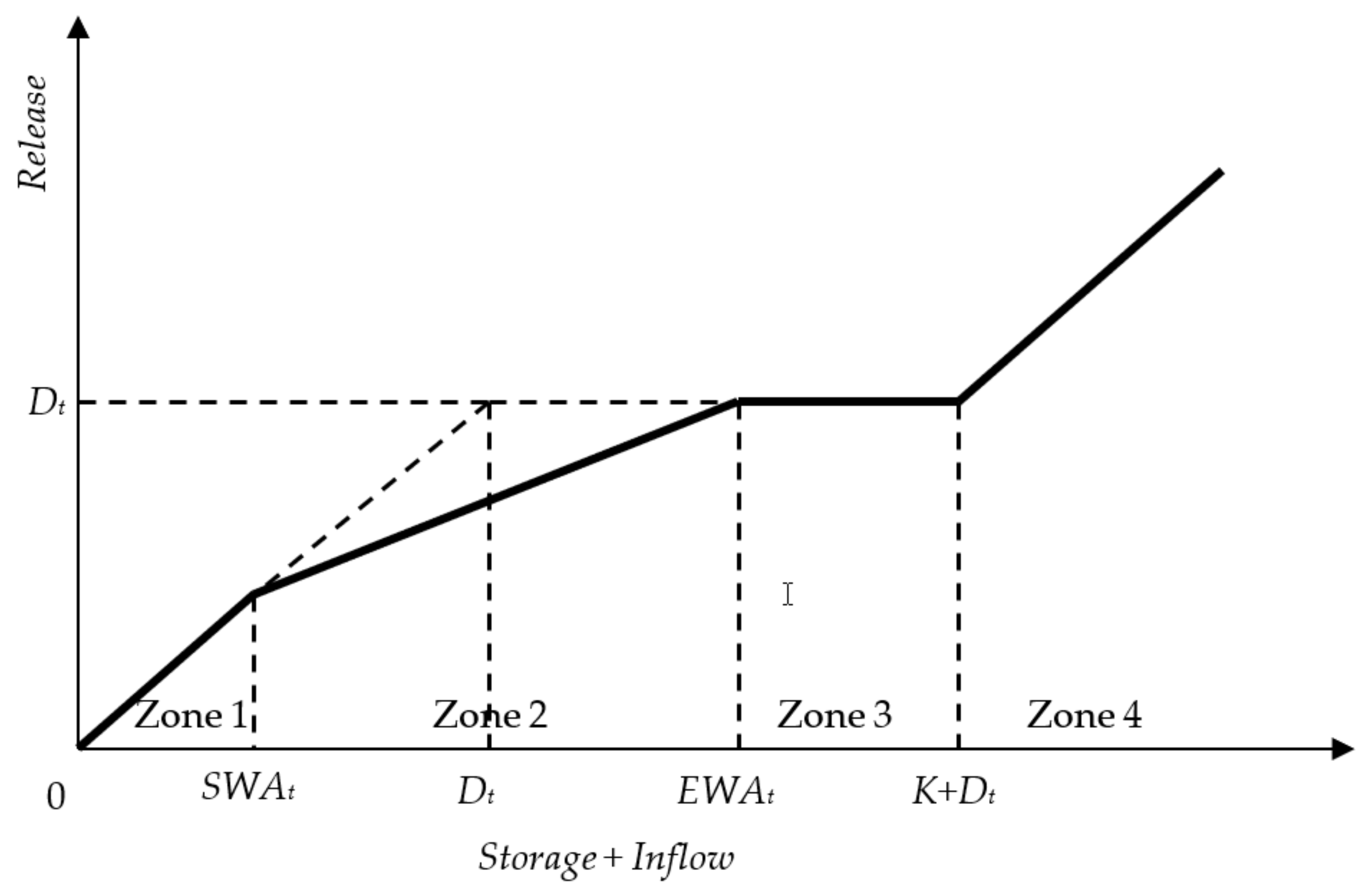
Bayzit and Unal [2] developed two-point linear hedging rule (Figure 1), in which, when the water availability falls below the starting water availability (SWA), the available water is released to satisfy the demand, which leads the reservoir storage to zero. If the water availability is greater than the ending water availability (EWA), hedging is stopped and normal operation is resumed. In case of water availability is between SWA and EWA, the hedging is applied and partial demand is satisfied in order to increase the storage (anticipating low flows in the future). Once the available water is more than ending water availability, hedging is stopped and normal operation is resumed.

$$A{W}_t=S_t+I_t$$

(5)

$$R_t=A{W}_t\mathrm{if}A{W}_t\le SW{A}_t$$

(6)

$$R_t=W{A}_t+\left(A{W}_t-SW{A}_t\right)\times \left(\frac{D_t-SW{A}_t}{EW{A}_t-SW{A}_t}\right)\mathrm{if}SW{A}_t\le A{W}_t\le EW{A}_t$$

(7)

$$R_t=D_t\mathrm{if}EW{A}_t\le A{W}_t\le K+D_t$$

(8)

$$R_t=D_t\mathrm{if}K+D_t\le A{W}_t$$

(9)

$$Spil{l}_t=\{\begin{array}{ll}A{W}_t-K-D_t& \mathrm{if}K+D_t\le A{W}_t\\ 0& \mathrm{else}\end{array}$$

(10)

$$S_{t+1}=S_t+I_t-R_t-Spil{l}_t$$

(11)

$$SW{A}_t=\alpha \times D_t$$

(12)

$$EW{A}_t=D_t+\left(K\times \beta \right)$$

(13)

In Equations (5)–(13), K is the reservoir capacity, AW_t denotes the available water during time period ‘t’, S_t denotes the initial storage, S_t+1 the final storage, R_t the release, and Q_t the inflows during time period ’t’. In the optimization formulation of the two-point hedging rule has two parameters α and β, which represents the starting water availability (SWA_t) and ending water availability (EWA_t), respectively.

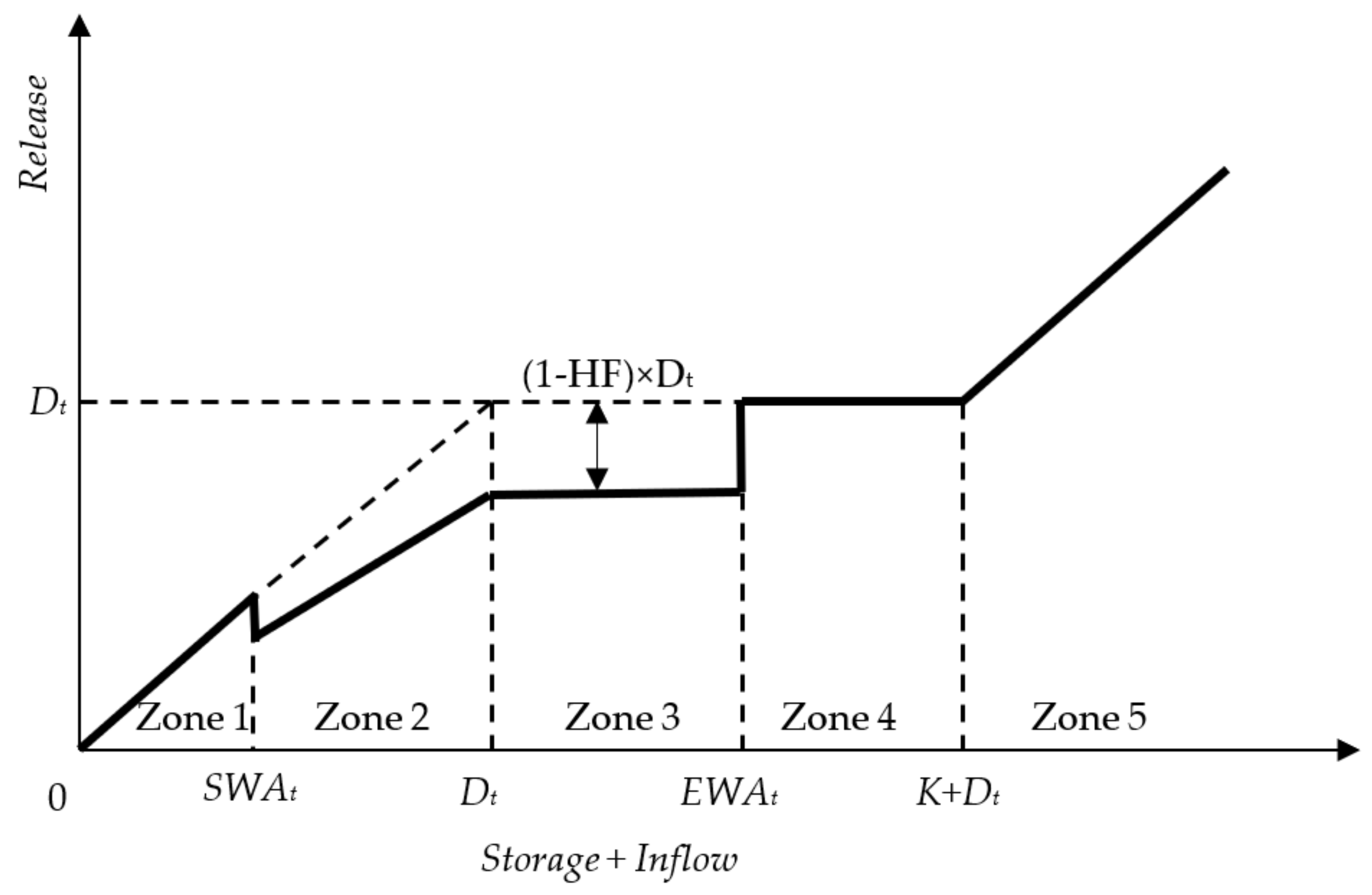
Srinivasan and Philipose [3,4], proposed a modified two-point hedging rule (Figure 2), in which the hedging factor (HF) specifies the amount of rationing to be done in addition to SWA and EWA. This answer the question “how much to hedge?” in addition to the starting and the ending periods of hedging.

$$A{W}_t=S_t+I_t$$

(14)

$$R_t=A{W}_t\mathrm{if}A{W}_t\le SW{A}_t$$

(15)

$$R_t=A{W}_t\left(1-HF\right)\mathrm{if}SW{A}_t\le A{W}_t\le D_t$$

(16)

$$R_t=D_t\left(1-HF\right)\mathrm{if}{D}_t\le A{W}_t\le EW{A}_t$$

(17)

$$R_t=D_t\mathrm{if}K+D_t\le A{W}_t$$

(18)

$$Spil{l}_t=\{\begin{array}{ll}A{W}_t-K-D_t& \mathrm{if}K+D_t\le A{W}_t\\ 0& \mathrm{else}\end{array}$$

(19)

$$S_{t+1}=S_t+I_t-R_t-Spil{l}_t$$

(20)

$$SW{A}_t=\alpha \times D_t$$

(21)

$$EW{A}_t=D_t+\left(K\times \beta \right)$$

(22)

$$0\le HF\le 1$$

(23)

In Equations (14)–(23), K is the reservoir capacity, AW_t denotes the available water during time period ‘t’, S_t denotes the initial storage, S_t+1 the final storage, R_t the release, and Q_t the inflows during time period ‘t’. In the optimization formulation of the modified two-point hedging rule, has three decision variables namely α, β, and HF.

2.1.3. Discrete Hedging Rule

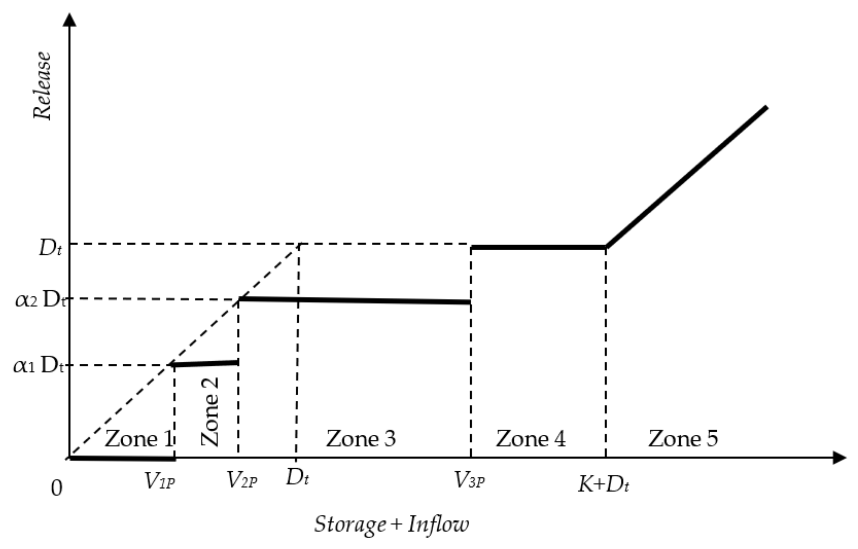
Shih and Revelle [9] proposed the discrete hedging scheme in which rationing is done on demand two phases based on the available water, as presented in Figure 3. In this rule, the trigger volumes of available water are introduced, where k₁, k₂, k₃ are the coefficients used to calculate V_1p, V_2p, V_3p, respectively.

$$A{W}_t=S_t+I_t$$

(24)

$$R_t=0\mathrm{if}A{W}_t\le V_{1p}$$

(25)

$$R_t={\alpha }_1\times D_t\mathrm{if}{V}_{1p}\le A{W}_t\le V_{2p}$$

(26)

$$R_t={\alpha }_2\times D_t\mathrm{if}{V}_{2p}\le A{W}_t\le V_{3p}$$

(27)

$$R_t=D_t\mathrm{if}{V}_{3p}\le A{W}_t\le K$$

(28)

$$R_t=D_t\mathrm{if}A{W}_t\ge K$$

(29)

$$Spil{l}_t=\{\begin{array}{ll}A{W}_t-K-D_t& \mathrm{if}K+D_t\le A{W}_t\\ 0& \mathrm{else}\end{array}$$

(30)

$$S_{t+1}=S_t+I_t-R_t-Spil{l}_t$$

(31)

$$V_{1p}=k_1\times D_t$$

(32)

$$V_{2p}=k_2\times D_t$$

(33)

$$V_{3p}=D_t+\left(k_3\times \left(K-D_t\right)\right)$$

(34)

$$0\le {\alpha }_1\le 1$$

(35)

$$0\le {\alpha }_2\le 1$$

(36)

$$k_1\ge {\alpha }_1$$

(37)

$$k_2\ge {\alpha }_2$$

(38)

$${\alpha }_2\ge {\alpha }_1$$

(39)

$$0\le k_1,k_2,k_3\le 1$$

(40)

$$k_2\ge k_1$$

(41)

2.2. Performance Evaluation

The PSO framework will provide a number of pareto-optimal solutions corresponding to each of the three hedging rules that are invoked. These pareto-optimal solutions that were obtained from the framework need to be evaluated in detail for their operational performance over the time horizon considered while using the reservoir simulation module. For the reservoir performance evaluation over the operation horizon, the following performance indicators are computed.

(i)

Occurrence-based reliability, the ratio of the number of times the demand is satisfied to the number of times the reservoir is operated [7].

(ii)

Resilience, the ratio of the number of times the system moved from failure to success to the total number of periods the system was in a failure state [7].

(iii)

Mean event deficit, the ratio of the total deficit volume encountered during the operation horizon to the total number of failure events. Herein, ‘event’ denotes a sequence of failure periods. The high magnitude of event deficit encountered during an irrigation season is detrimental to crop yield.

(iv)

Event vulnerability is the maximum event deficit that is encountered during the operation horizon of the reservoir.

2.3. Solution Technique

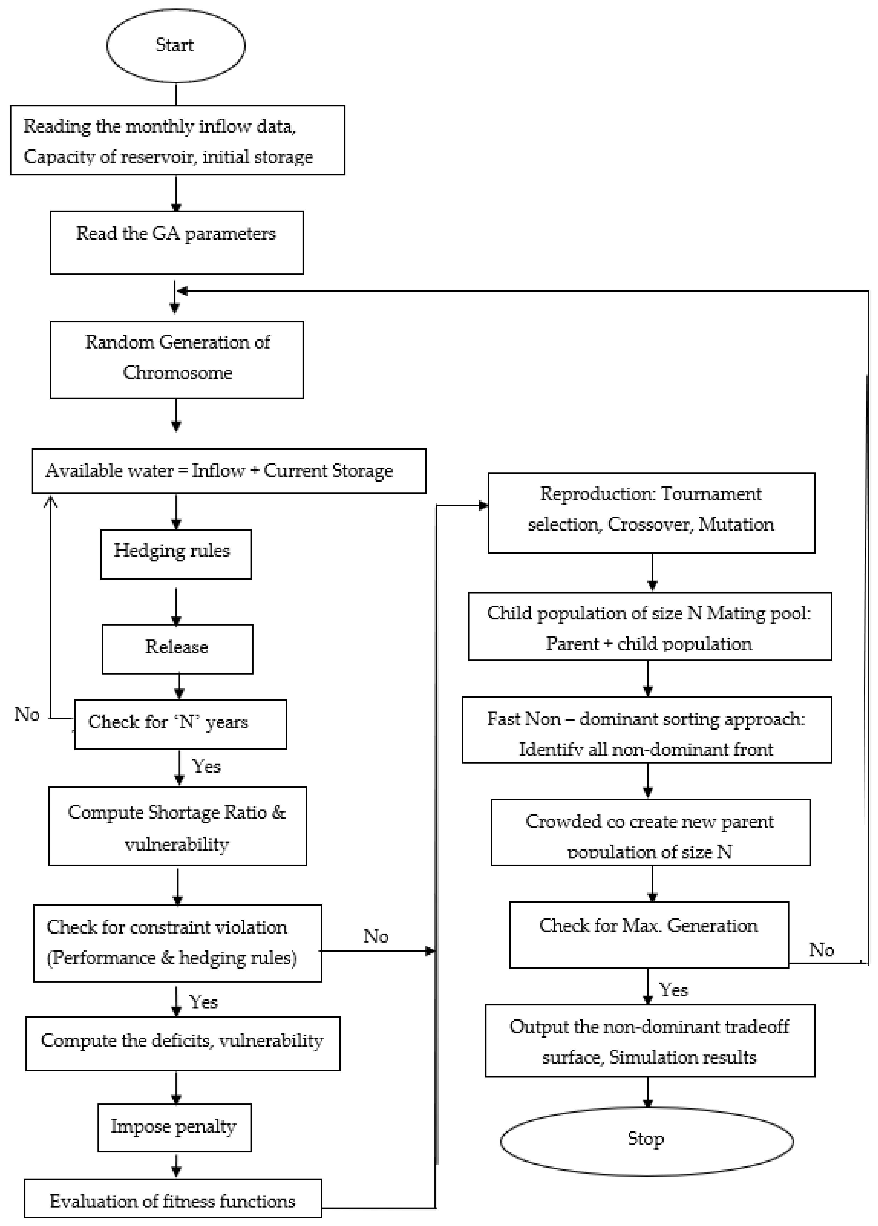
The technique adopted in this research work to solve the multi-objective optimization problem is the Non-dominated Sorting Genetic Algorithm-II (NSGA-II), as proposed by Deb et al. [27]. This technique is known to be better than the traditional multi-objective optimization methods such as ε -constraint method, weighted sum method in generating near-global pareto-optimal fronts. This technique is suited for handling complex objective functions involving discontinuities, disjoint feasible spaces, and noisy function evaluations [28]. The multi-objective optimization model is the driver and the simulation model that is based on the hedging rules forms the engine of the framework. The decision variables of the optimization model are the hedging rule parameters. The strings that are generated from NSGA-II are evaluated for the two fitness functions while using the simulation model. The near-(global) optimal search is based on the “survival of the fittest” principle of the evolution theory. The improvements in the quality of the solutions are achieved through the genetic operators, selection, crossover, and mutation. Elitist-based Non-dominated sorting, tournament selection, and crowded comparison operator are a few of the special features that were implemented into NSGA-II to enhance its speed, quality and diversity of the non-dominated solutions. The Multi-Objective Genetic Algorithm (MOGA) input requirements are population size, number of generations, crossover probability, mutation probability, and random seed. The other inputs that are required for running the simulation module are inflows into the reservoir irrigation demands and the physical characteristics of the reservoir and the choice of the hedging rule for the operation of the reservoir. The illustration of the framework, including the steps involved in NSGA-II, is presented in Appendix A.

2.4. Case Study—Hemavathy Reservoir

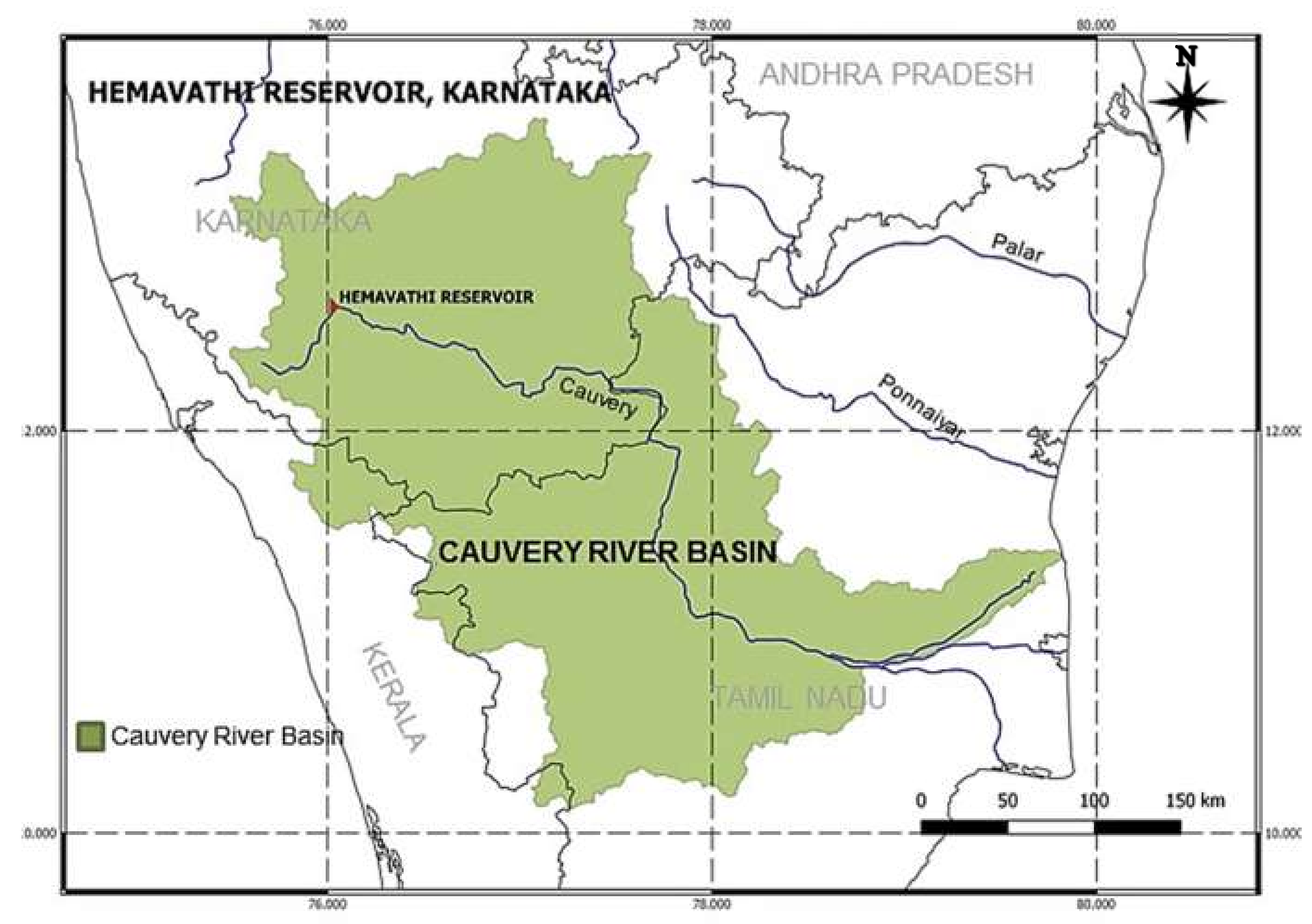
The reservoir performance for the three selected hedging policies based on the PSO framework is evaluated using Hemavathy Reservoir, located in the Upper Cauvery River Basin, in Southern India (Figure 4). The salient features of the reservoir are: (i) total catchment area of 5910 km²; (ii) gross storage capacity is 1048 Mm³; and, (iii) live storage capacity of 962.77 Mm³. In this study, we used monthly inflows and irrigation demands for the reservoir operation model (

Table 1. Mean monthly inflows and monthly target yields of River Hemavathy.

Month	June	July	August	September	October	November	December	January	February	March	April	May
Mean Monthly Inflow (Mm3)	150	856	665	296	285	127	55	30	18	14	14	36
Target Yield (Mm3)	165	260	275	75	50	120	280	350	225	80	20	10

). It can be observed from Table 1 that most of the inflows are received between the months of June and November (~93%). While the remaining months receives less than 10% of the total annual flow. Further, it is to be noted that the reservoir storage exhibits a with-in year behavior, i.e., both filling and emptying occurs within the operating year. A data set for a period of 58 years is used for the present study. For more details about the reservoir salient features and inflow and demand characteristics, the readers are referred to [3].

3. Results and Discussion

In this study, the efficacy of the time-varying (TV) hedging (TVH) is compared with that of the constant hedging (CH) for three selected hedging policies, namely, two-point hedging (TPH), modified two-point hedging (MTPH), and discrete hedging (DH). This results in a total of six cases are used for the comparison studies (

Table 2. The list of hedging models (with acronyms) used for comparison.

	Two-Point Hedging (TPH)	Modified Two-Point Hedging (MTPH)	Discrete Hedging (DH)
Time-Varying	TV-TPH	TV-MTPH	TV-DH
Constant	C-TPH	C-MTPH	C-DH

). The performance of each of the hedging policies has been evaluated using various indices, such as period vulnerability, shortage ratio, occurrence reliability, volume reliability, and resilience. In addition, the results are presented for three critical demand levels, namely 75%, 80%, and 85% of the mean annual flow.

3.1. Selection of GA Parameters

For the three hedging policies that are considered in this study, sensitivity analysis is carried out on NSGA-II parameters, namely, number of generations, population size, mutation probability, cross-over probability, and random seed. Table 2 provides the details of the range of parameters considered and the selected parameters that are based on the inter-comparison of the Pareto-optimal fronts. It is observed from Table 2 that the population size (100), number of generations (300), and mutation probability (0.01) remained constant for all of the hedging policies and across all the demand levels. However, the cross-over probability and random seed are found to be sensitive in obtaining the near optimal pareto-fronts and vary with hedging policies (

Table 3. Selected genetic algorithm (GA) parameters based on the sensitivity analysis for time-varying hedging policies (two-point hedging (TPH), modified two-point hedging (MTPH), and discrete hedging (DH)).

GA Parameter	Range	Selected Parameter
		Two-Point Hedging (TV-TPH)			Modified Two-Point Hedging (TV-MTPH)			Discrete Hedging (TV-DH)
Demand %		75	80	85	75	80	85	75	80	85
Population	50,100,200	100	100	100	100	100	100	100	100	100
Generation	100,300,500	300	300	300	300	300	300	300	300	300
Cross Over	0.6,0.7,0.8,0.9	0.7	0.8	0.9	0.8	0.7	0.7	0.6	0.7	0.7
Mutation	0.001,0.005,0.01	0.001	0.001	0.001	0.001	0.001	0.001	0.001	0.001	0.001
Random Seed	0.25,0.35,0.45 0.55,0.65,0.75	0.65	0.45	0.45	0.75	0.25	0.25	0.65	0.25	0.45

).

3.2. Comparison of Time-Varying and Constant Hedging Policies

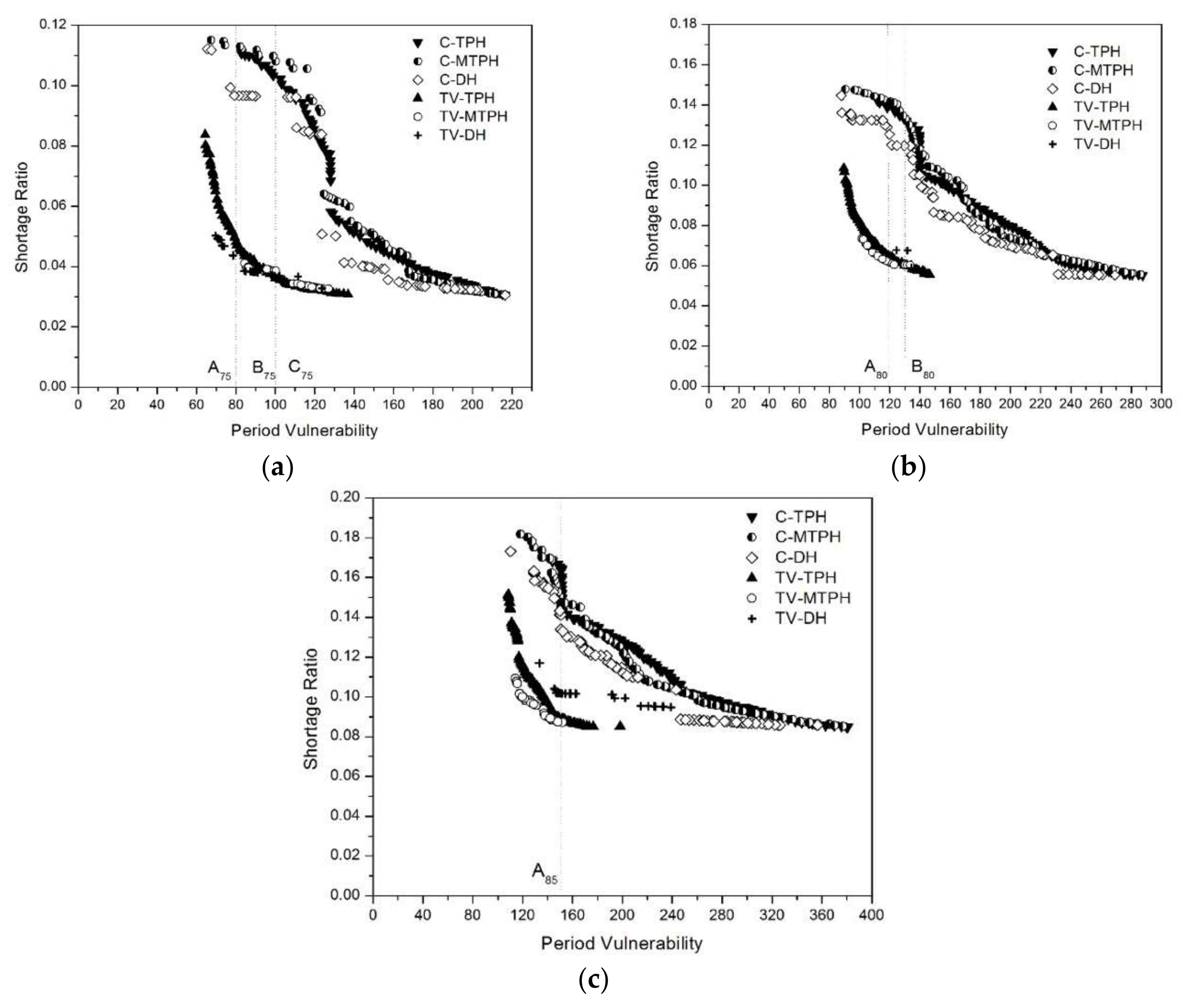
The pareto-optimal fronts comparing the variation of selected best hedging policies for both the constant and time-varying hedging parameters are presented in Figure 5. It is evident from the Figure 5 that the time-varying hedging policies are found to perform better in comparison to the constant hedging policies at all demand levels that are considered in this study. However, the constant hedging policies produce a wider range of pareto-optimal solutions when compared to the time-varying hedging policies. In the case of time-varying hedging policies, TV-TPH has more range of pareto-optimal solutions when compared to TV-MTPH and TV-DH. Further, the relative performance of the TV-DH decreases as the demand level increases.

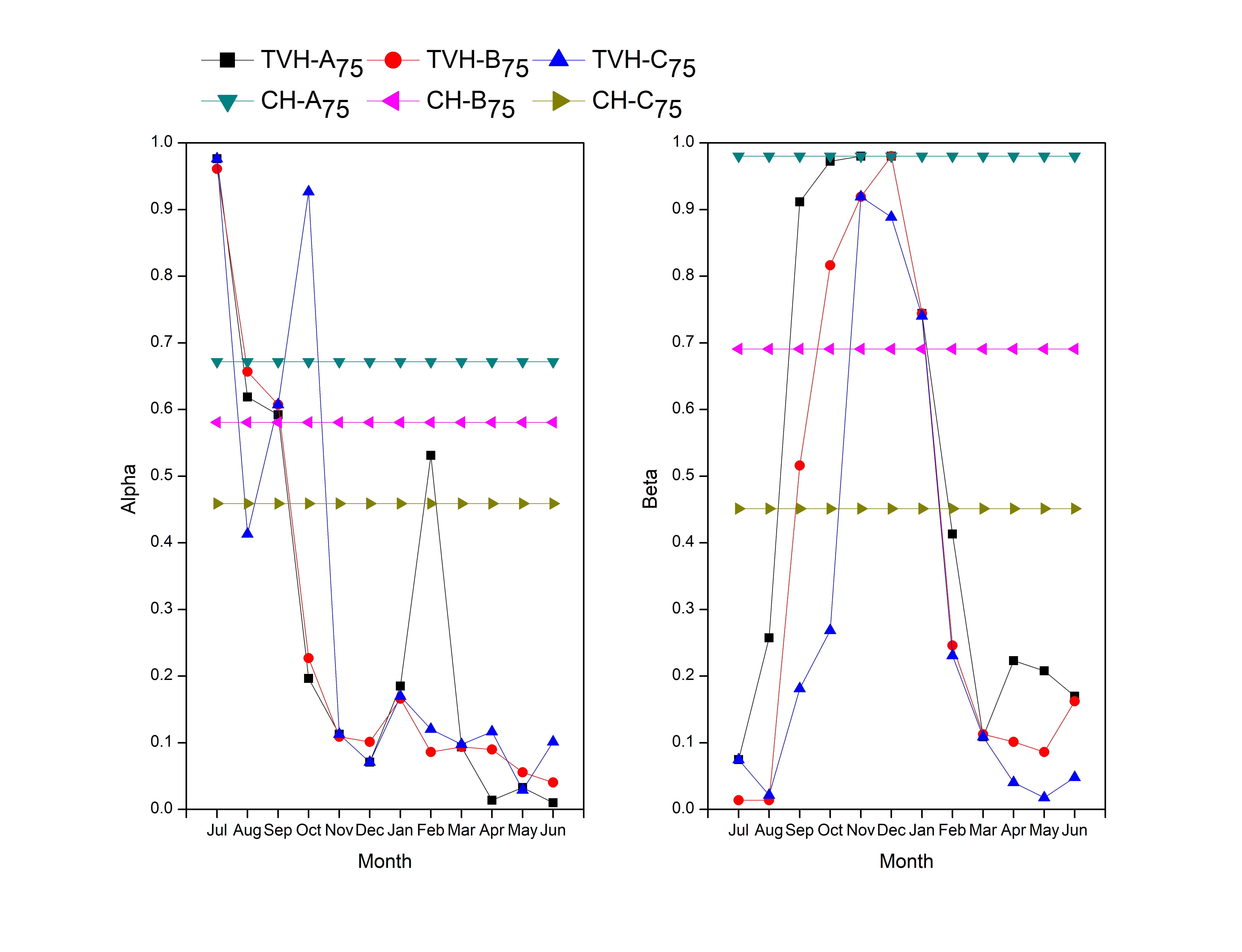
The detailed comparison of the performance indicators that were adopted in this study for each of the hedging policies is presented in

Table 4. Reservoir performance indices at 75% demand level for two point linear—a comparison of time-varying and constant hedging policies for selected compromising solutions (see figure 5).

	Period Vulnerability	Shortage Ratio	Volume Reliability	Occurrence Reliability	Resilience	Mean Event Deficit	Number of Period Deficits
SOP	216.58	0.031	0.969	0.93	0.51	135.2	49
Time-Varying Hedging
TV-Max S/R	64.44	0.084	0.916	0.461	0.275	89.89	376
TV-Max Vul	136.97	0.031	0.969	0.841	0.387	79.2	111
TV-A75	80.01	0.048	0.952	0.595	0.355	53.24	282
TV-B75	102.08	0.036	0.964	0.728	0.344	61.12	189
TV-C75	119.23	0.032	0.968	0.829	0.479	62.47	119
Constant Hedging
C-Max S/R	82.81	0.111	0.889	0.389	0.134	215.61	426
C-Max Vul	216.58	0.031	0.969	0.917	0.431	135.23	58
C-A75	82.81	0.111	0.889	0.389	0.134	215.61	426
C-B75	98.78	0.103	0.897	0.428	0.143	200.48	399
C-C75	120.56	0.084	0.916	0.501	0.164	163.29	347

,

Table 5. Reservoir performance indices at 75% demand level for modified two point linear—a comparison of time-varying and constant hedging policies for selected compromising solutions (see figure 5).

	Period Vulnerability	Shortage Ratio	Volume Reliability	Occurrence Reliability	Resilience	Mean Event Deficit	Number of Period Deficits
SOP	216.58	0.031	0.969	0.93	0.51	135.2	49
Time-Varying Hedging
TV-Max S/R	84.45	0.041	0.959	0.865	0.606	79.75	94
TV-Max Vul	126.95	0.033	0.967	0.911	0.709	81.96	62
TV-A75	84.45	0.041	0.958	0.865	0.606	79.75	94
TV-B75	100.34	0.039	0.961	0.904	0.716	89.08	67
TV-C75	119.99	0.033	0.967	0.899	0.714	73.36	70
Constant Hedging
C-Max S/R	67.41	0.115	0.885	0.395	0.133	227.33	422
C-Max Vul	214.72	0.031	0.969	0.917	0.431	135.75	58
C-A75	82.14	0.113	0.887	0.402	0.135	223.16	417
C-B75	100.21	0.108	0.892	0.391	0.13	217.32	425
C-C75	119.05	0.095	0.905	0.579	0.198	180.76	293

and

Table 6. Reservoir performance indices at 75% demand level for discrete hedging—a comparison of time-varying and constant hedging policies for selected compromising solutions (see figure 5).

	Period Vulnerability	Shortage Ratio	Volume Reliability	Occurrence Reliability	Resilience	Mean Event Deficit	Number of Period Deficits
SOP	216.58	0.031	0.969	0.93	0.51	135.2	49
Time-Varying Hedging
TV-Max S/R	69.57	0.05	0.95	0.79	0.74	51.52	146
TV-Max Vul	123.61	0.033	0.967	0.856	0.43	84.19	100
TV-A75	78.53	0.044	0.956	0.866	0.7	74.2	93
TV-B75	98.35	0.037	0.963	0.888	0.628	83.76	78
TV-C75	123.61	0.033	0.967	0.856	0.43	84.19	100
Constant Hedging
C-Max S/R	65.59	0.112	0.888	0.394	0.133	221.6	423
C-Max Vul	216.58	0.03	0.969	0.922	0.5	125.28	54
C-A75	79.18	0.097	0.903	0.395	0.128	198.02	422
C-B75	106.22	0.096	0.904	0.402	0.132	193.44	417
C-C75	123.5	0.084	0.916	0.46	0.152	162.81	377

. For brevity, the results for the 75% demand level is presented here, as the similar performance was observed for the other demand levels. The results for the 80% and 85% demand levels are provided for the readers as supplementary material (Figure S1–S6 and Table S1–S6). The pareto-front for each of the hedging models contains 100 possible trade-off solutions. For brevity few solutions from the pareto-front are selected for comparison of the hedging policies. The selection includes: (i) two extreme solutions related to the maximum shortage ratio and maximum vulnerability and (ii) three intermediate solutions which includes the solution closest to the origin (i.e., the best trade-off solution). It is to be noted that, in few cases, the number of feasible solutions show limited range due to restricted parameter search space. In such instances, the number of intermediate solutions is restricted to one or two intermediate solutions depending on the available range of pareto-front. In this study, for comparison, three intermediate solutions (TV-A75, TV-B75, TV-C75) and two extreme solutions that include minimum vulnerability (or maximum shortage ratio) (TV-Max S/R) and minimum shortage ratio (or maximum vulnerability) (TV-Max Vul) for the 75% demand level are selected from the pareto-optimal fronts. Further, these results are compared with the performance of the standard operating policy (SOP).

It is observed from Table 4, Table 5 and Table 6, that the hedging policies perform better when compared to SOP in terms of reducing the period vulnerability of reservoir operation. It is to be noted that the SOP does not account for the low reservoir inflows, and hence resulting in larger vulnerabilities. In addition, the hedging policies reduce the overall shortages by increasing the number of deficit periods when compared to SOP (which has higher shortages and lower number of deficits). From the Table 4, Table 5 and Table 6, it is evident that the time-varying hedging policies show considerable improvement in reservoir performance indicators when compared to the constant hedging policies. Further, the time-varying hedging rules produces relatively lower vulnerability, shortage ratio, and mean event deficit when compared to constant hedging rules. For the selected solutions (A, B, C), the time-varying hedging (TVH) policies show (relatively) decrease in shortage ratio by 60% and mean event deficit by 68%. In addition, the TVH policies show an average increase in volume reliability and occurrence reliability by 6% and 65% respectively. However, the resilience of the TVH is more than the CH, which indicates that the length of the events is longer when compared to the CH. It is to be noted that TVH is able to improve the performance of the long-term reservoir operation by having longer low volume (event) deficits when compared to shorter high volume (event) deficits by CH or SOP. The better performance of the TVH polices is due to the significant decrease in number of deficit periods occurred and mean event deficit during the entire reservoir simulation period when compared to CH. It is to be noted that the significant decrease in deficit periods could be explained by the time-varying hedging/rationing parameters of the policies. The variation of hedging parameters for the selected cases is presented in the following paragraphs.

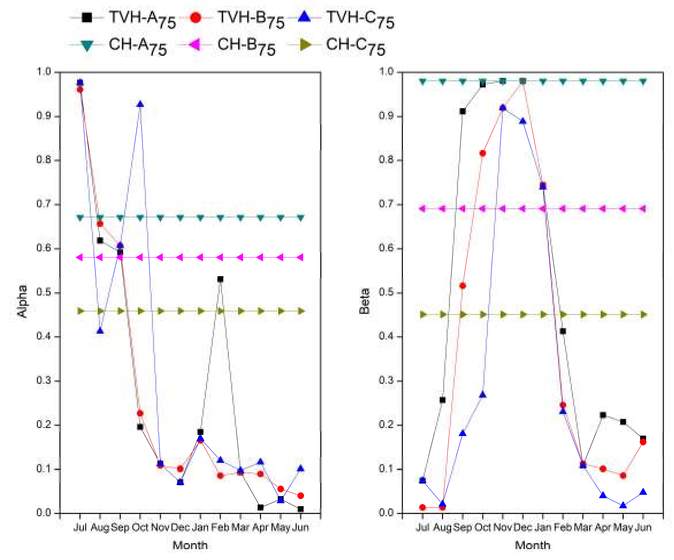
The variation of the three hedging parameters for 75% demand levels are presented in Figure 6, Figure 7 and Figure 8. The following points are observed

(i)

The CH parameters are higher in many months when compared to TVH parameters, i.e., the hedging factors (rationing as well as storage levels-based factors) are higher. For example, in the case of two-point hedging policy (Figure 6): higher vulnerability solution (C-A₇₅) the rationing is carried out even though the reservoir storage levels are high.

(ii)

For TV-TPH (Figure 6) it is observed that for the months April to August, the release is marginally different from SOP, i.e., the deficits are minimized by utilizing the maximum available water from the reservoir. It is evident from Figure 6 that the TVH parameters are adaptable to hedge the available water from high inflow months and carry-over the same during the low-flow months when compared to CH. In CH, although the hedging is carried out during the high-flow months, due to constant parameters, it is forced to continue hedging in low-flow periods, resulting in higher volume of deficits.

(iii)

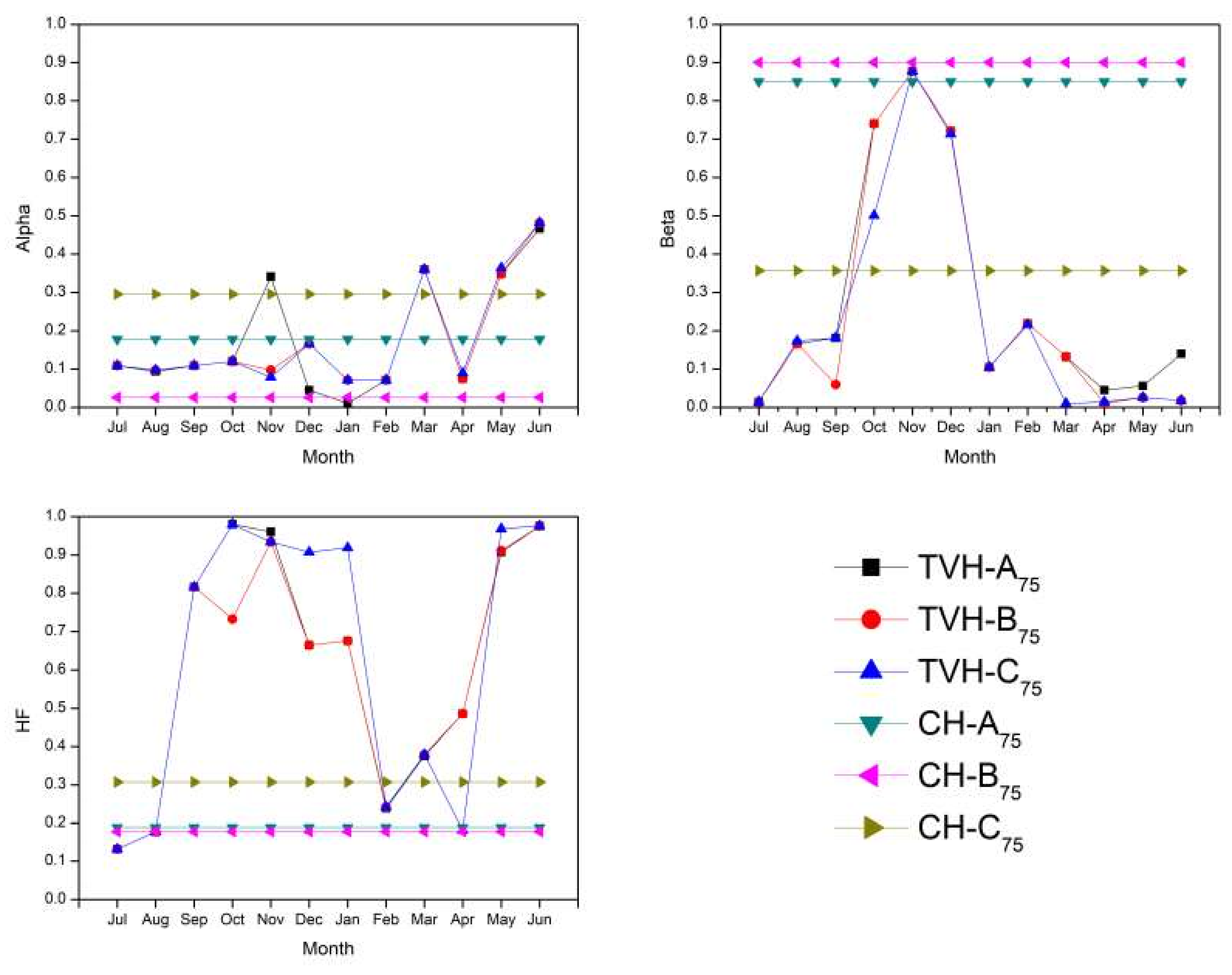
Similarly it is observed from Figure 7, that for MTPH most of the dry months TVH parameters have low hedging factors, indicating that those months are simulated as a SOP. The rationing is carried out during high inflow months and low storage levels as contradictory to constant hedging policies.

(iv)

In case of MTPH, the additional rationing factor HF plays a significant role in the variation of parameters alpha and beta. It is observed from Figure 7 that the rationing factor is higher in case of CH when compared to TVH, except for few months. In case of TVH, during October-January and April-May is simulated as two-point hedging rule. It is noted that, due to time-varying parameters in MTPH, it is able to efficiently hedge in demand (HF) and/or storage (alpha and beta), unlike the CH. This could be one of the plausible reasons for MTPH to perform better when compared to TPH. Further it is the variation of beta in both TPH and MTPH are similar, however MTPH alpha is significantly different from TPH. This shows that starting water availability is significantly affected by the rationing factor.

(v)

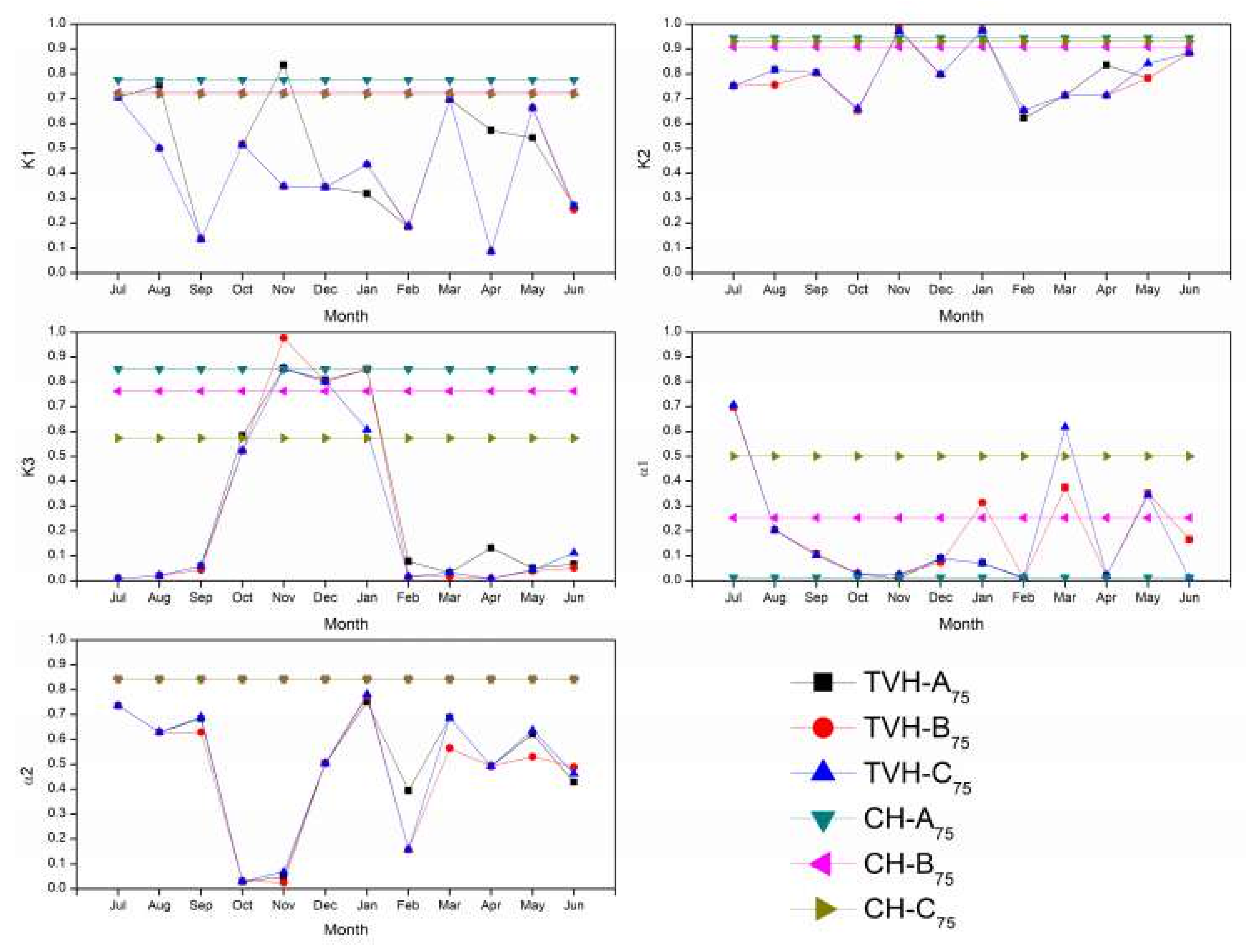
It is observed from Figure 8, that, for discrete hedging policy, the time-varying parameters are significantly different for all of the months in comparison to constant hedging. The K₃ parameter is has similar trend to beta parameter of TVH and MTPH.

(vi)

It is evident that, most of the rationing for CH is carried out in zones 1, 2, and 3. However, the TVH the rationing factors are dominant in high flow months when compared to low flow months. Therefore, the TVH is able reduce the number of failure events when compared to CH.

In addition, it is observed that the variation of the parameters for the selected pareto solutions for TVH in most of the dry months is insignificant. However, in high flow months, there is considerable variation in the parameters. Further, the parameters that are related to storage levels have more impact on the performance of the reservoir in comparison to the rationing parameters.

4. Summary and Conclusions

The study examined the performance of the reservoir simulation model while using time-varying hedging (TVH) policies and compared with the constant hedging (CH) policies. A parameterization-simulation-optimization (PSO) framework is used for obtaining compromising hedging policies for the operation of a reservoir. These hedging policies seek to obtain the trade-off between minimizing shortage ratio and minimizing vulnerability, which are the two primary objectives of a water manager for the operation of a reservoir during droughts. The NSGA-II algorithm is adopted as an optimization tool. The performance comparison is carried out for three commonly used hedging rules for reservoir operation. The case example that is used for illustration is the operation of the Hemavathy reservoir, Southern India. The following conclusions are drawn from this research:

(i)

The sensitivity analysis on NSGA-II parameters indicated that the cross-over probability and random seed are found to be sensitive when compared to population size, number of generations, and mutation probability.

(ii)

Both the TVH and CH yield better alternative solutions in comparison to SOP, in terms of lower period vulnerabilities and shortage ratios.

(iii)

The reservoir performance has significantly increased with TVH when compared to CH.

(iv)

The decrease in number of deficits and mean period vulnerability are the key factors for better performance of the TVH

(v)

The hedging parameters for TVH indicate less rationing in low reservoir inflows and lower storage levels when compared to CH rationing, which is constant irrespective of inflows and storage levels.

References

- Draper, A.J.; Lund, J.R. Optimal hedging and carryover storage value. J. Water Resour. Plann. Manag. 2004, 130, 83–87. [Google Scholar] [CrossRef]
- Bayazit, M.; Unal, N.E. Effects of hedging on reservoir performance. Water Resour. Res. 1990, 26, 713–719. [Google Scholar] [CrossRef]
- Srinivasan, K.; Philipose, M.C. Evaluation and Selection of Hedging policies using stochastic Reservoir Simulation. Water Resour. Manag. 1996, 10, 163–188. [Google Scholar] [CrossRef]
- Srinivasan, K.; Philipose, M.C. Effect of hedging on over-year reservoir performance. Water Resour. Manag. 1998, 12, 95–120. [Google Scholar] [CrossRef]
- You, J.Y.; Cai, X. Hedging Rules for reservoir operations 1. A theoretical analysis. Water Resour. Res. 2008, 44, W01415. [Google Scholar] [CrossRef]
- You, J.Y.; Cai, X. Hedging rule for reservoir operations: 2. A numerical model. Water Resour. Res. 2008, 44, W01416. [Google Scholar] [CrossRef]
- Hashimoto, T.; Stedinger, J.R.; Loucks, D.P. Reliability, resiliency, and vulnerability criteria for water resources system evaluation. Water Resour. Res. 1982, 18, 14–20. [Google Scholar] [CrossRef]
- Shih, J.; ReVelle, C. Water-Supply Operations During Drought: Continuous Hedging Rule. J. Water Resour. Plan. Manag. 1994, 120, 613–629. [Google Scholar] [CrossRef]
- Shih, J.-S.; ReVelle, C. Water Supply Operations During Drought: A Discrete Hedging Rule. Eur. J. Oper. Res. 1995, 82, 163–175. [Google Scholar] [CrossRef]
- Neelakantan, T.R.; Pundarikanthan, N.V. Hedging rule optimization for water supply reservoirs system. J. Water Resour. Plann. Manag. 1999, 13, 409–426. [Google Scholar] [CrossRef]
- Shiau, J.T.; Lee, H.C. Derivation of optimal hedging rules for a water supply reservoir through compromise programming. Water Resour. Manag. 2005, 19, 111–132. [Google Scholar] [CrossRef]
- Celeste, A.B.; Billib, M. Evaluation of stochastic reservoir operation optimization models. Adv. Water Resour. 2009, 32, 1429–1443. [Google Scholar] [CrossRef]
- Oliveira, R.; Loucks, D. Operating rules for multi-reservoir systems. Water Resour. Res. 1997, 33, 839–852. [Google Scholar] [CrossRef]
- Srinivasan, K.; Kranthi, K. Multi-Objective Simulation-Optimization model for long-term reservoir operation using piecewise linear hedging rule. Water Resour. Manag. 2018, 32, 1901–1911. [Google Scholar]
- Liu, Y.; Zhao, J.; Hang, Z. Piecewise-linear hedging rules for reservoir operation with economic and ecologic objectives. Water 2018, 10, 865. [Google Scholar] [CrossRef]
- Neelakantan, T.R.; Pundarikanthan, N.V. Neural network-based simulation-optimization model for reservoir operation. J. Water Resour. Plan. Manag. 2000, 126, 57–64. [Google Scholar] [CrossRef]
- Sangiorgio, M.; Guariso, G. NN-Based Implicit Stochastic Optimization of Multi-Reservoir Systems Management. Water 2018, 10, 303. [Google Scholar] [CrossRef]
- Yi, J.; Lei, X.; Cai, S.; Wang, X. Hedging rules for water supply reservoir based on the model of simulation and optimization. Water 2016, 8, 249. [Google Scholar]
- Tu, M.N.; Hsu, N.S.; William, Y.G. Optimization of Hedging Rules for Reservoir Operations. J. Water Resour. Plan. Manag. 2008, 134, 3–13. [Google Scholar] [CrossRef]
- Shiau, T.J. Optimization of Reservoir Hedging Rules Using Multiobjective Genetic Algorithm. J. Water Resour. Plan. Manag. 2009, 135, 355. [Google Scholar] [CrossRef]
- Shiau, J.T. Analytical optimal hedging with explicit incorporation of reservoir release and carryover storage targets. Water Resour. Res. 2011, 47. [Google Scholar] [CrossRef] [Green Version]
- Wang, H.; Liu, J. Reservoir Operation Incorporating Hedging Rules and Operational Inflow Forecasts. Water Resour. Manag. 2013, 27, 1427–1438. [Google Scholar] [CrossRef]
- Spiliotis, M.; Luis, M.; Luis, G. Optimization of Hedging Rules for Reservoir Operation During Droughts Based on Particle Swarm Optimization. Water Resour. Manag. 2016, 30, 5759–5778. [Google Scholar] [CrossRef]
- Xu, B.; Zhong, P.-A.; Huang, Q.; Wang, J.; Yu, Z.; Zhang, J. Optimal Hedging Rules for Water Supply Reservoir Operations under Forecast Uncertainty and Conditional Value-at-Risk Criterion. Water 2017, 9, 568. [Google Scholar] [CrossRef]
- Koutsoyiannis Demetris; Athanasia Economou. Evaluation of the parameterization-simulation-optimization approach for the control of reservoir systems. Water Resour. Res. 2003, 39, 1170. [Google Scholar]
- Giuliani, M.; Emanuele, M.; Andrea, C.; Francesca, P.; Rodolfo, S. Universal approximators for direct policy search in multi-purpose water reservoir management: A comparative analysis. In Proceedings of the 19th World Congress, The International Federation of Automatic Control, Cape Town, South Africa, 24–29 August 2014; pp. 6234–6239. [Google Scholar]
- Deb, K.; Pratap, A.; Agarwal, S.; Meyarivan, T. A Fast and Elitist Multiobjective Genetic Algorithm: NSGA-II. IEEE Trans. Evolut. Comput. 2002, 6, 182–197. [Google Scholar] [CrossRef]
- Fonseca, C.M.; Fleming, P.J. An overview of evolutionary algorithms in multi-objective optimization. Evolut. Comput. 1995, 3, 1–16. [Google Scholar] [CrossRef]
Figure 1.
Two-point hedging policy (SWAt—Starting Water availability; EWAt—Ending Water availability; Dt—Demand; and, t denotes the time period).
Figure 2.
Modified two-point hedging policy (SWAt—Starting Water availability, EWAt—Ending Water availability, Dt—Demand, HF–Hedging Factor; and, t denotes the time period). Modified two-point hedging rule.
Figure 3.
Discrete hedging policy (Dt—demand, α1, α2-rationing factor; and, t denotes time period).
Figure 4.
Location of Hemavathi Reservoir – Upper Cauvery Basin. Blue line indicates the river network.
Figure 5.
Pareto fronts for two point linear hedging, modified two point hedging and discrete hedging at 75%, 80% and 85% demand levels—Comparison of time-varying and constant hedging.
Figure 6.
Time-varying hedging (TVH) and constant hedging (CH) parameters (alpha and beta) for two-point hedging policy—A comparison between the selected pareto-optimal solutions for 75% demand level.
Figure 7.
Time-varying hedging (TVH) and constant hedging (CH) parameters (alpha, beta and hedging factor) for modified two-point hedging policy—A comparison between the selected pareto-optimal solutions for 75% demand level.
Figure 8.
Time-varying hedging (TVH) and constant hedging (CH) parameters (K1, K2, K3, α1, α2) for discrete hedging policy—A comparison between the selected pareto-optimal solutions for 75% demand level.