

Abstract
Permafrost temperatures are increasing globally with the potential of adverse environmental and socio-economic impacts. Nonetheless, the attribution of observed permafrost warming to anthropogenic climate change has relied mostly on qualitative evidence. Here, we compare long permafrost temperature records from 15 boreholes in the northern hemisphere to simulated ground temperatures from Earth system models contributing to CMIP6 using a climate change detection and attribution approach. We show that neither pre-industrial climate variability nor natural drivers of climate change suffice to explain the observed warming in permafrost temperature averaged over all boreholes. However, simulations are consistent with observations if the effects of human emissions on the global climate system are considered. Moreover, our analysis reveals that the effect of anthropogenic climate change on permafrost temperature is detectable at some of the boreholes. Thus, the presented evidence supports the conclusion that anthropogenic climate change is the key driver of northern hemisphere permafrost warming.
Export citation and abstract BibTeX RIS

Original content from this work may be used under the terms of the Creative Commons Attribution 4.0 license. Any further distribution of this work must maintain attribution to the author(s) and the title of the work, journal citation and DOI.
1. Introduction
Permafrost, a subsurface feature of polar and alpine regions, is defined as ground that remains at or below 0 °C for many years. Permafrost influences the functioning of natural and human systems in high latitude and high altitude landscapes. State of the art Earth system models (ESM) unanimously project massive reductions in permafrost occurrence in response to man-made global warming (Burke et al 2020), which is particularly pronounced in polar and high mountain regions. This implies an increasing risk of permafrost warming and degradation with far-reaching consequences for both local environments and Earth system dynamics (IPCC 2019). For example, permafrost stores approximately twice as much carbon as the Earth's atmosphere currently holds (Schuur et al 2009). Through processes known as the permafrost carbon feedback, a breakdown of organic carbon associated with permafrost degradation has the potential to release large amounts of greenhouse gases into the atmosphere and thus further contribute to global warming (Schuur et al 2015). Moreover, permafrost degradation can have significant effects on vegetation (Jin et al 2021) and tundra hydrology (Liljedahl et al 2016), damage infrastructure (Hjort et al 2018, Duvillard et al 2019), or impede winter overland transport (Gädeke et al 2021). In steep environments, permafrost warming has been associated with increasing magnitude and frequency of alpine mass movements such as rockfalls (Gruber and Haeberli 2007, Ravanel and Deline 2010, Marcer et al 2021).
Observational studies have documented systematic change of permafrost thermal state in recent years. For example, permafrost ground temperatures have been shown to increase at regional (Etzelmüller et al 2020, Vasiliev et al 2020, Zhao et al 2020, Haberkorn et al 2021, Smith et al 2021) and global scales (Biskaborn et al 2019, Hock et al 2019, Noetzli et al 2020, Smith et al 2022). The main driver of permafrost warming is rising air temperature. But also additional heat introduced by precipitation (Mekonnen et al 2021) and effects related to changing snow insulation (Lawrence and Slater 2010) contribute. Permafrost warming is further modulated by ground properties, ground ice content, hydrology, or vegetation cover (Stuenzi et al 2021, Smith et al 2022).
Although permafrost warming is associated with rising air temperatures, the observed increase of permafrost temperature has to date not been unambiguously related to anthropogenic climate change. More precisely, it remains unclear whether increasing permafrost temperatures can be attributed to human-induced global warming or if natural climate variability is sufficient to explain the observed change. Such questions are addressed using climate change detection and attribution approaches, which are used for assessing impacts of anthropogenic emissions on the Earth's climate (Hegerl et al 2006, Bindoff et al 2013, Eyring et al 2021). Here the term detection refers to 'the process of demonstrating that an observed change is significantly different ... from natural internal climate variability' (Hegerl et al 2006). Furthermore, attribution of an observed change to human emissions includes a 'demonstration that the detected change is consistent with simulated change driven by ... anthropogenic changes in the composition of the atmosphere [e.g. greenhouse gas concentrations]..., and not consistent with alternative explanations of recent ... change...' (Hegerl et al 2006). Traditionally, the focus of detection and attribution studies was put on large-scale climate indicators, including global temperatures (Jones et al 2013) or zonal precipitation (Zhang et al 2007). However, an increasing number of studies have attributed changes in terrestrial systems including in river flow (Gudmundsson et al 2017, 2021), water availability (Padrón et al 2020), drought indicators (Marvel et al 2019) and global lake systems (Grant et al 2021) to man-made climate change. Addressing the question of permafrost warming at the global scale, Guo et al (2020) demonstrated that the observed change in an air temperature-based permafrost index is not consistent with natural factors and that human emissions need to be considered as an explanatory cause.
While previous assessments show that the atmospheric drivers affecting permafrost are shifting in response to human emissions (Guo et al 2020), it is still not clear to which extent the effect of anthropogenic climate change is detectable in direct permafrost temperature observations. An unambiguous attribution of trends in permafrost temperatures is complicated by three factors.
First, permafrost monitoring is based on in-situ ground temperatures measured in boreholes (Noetzli et al 2021). Their installation and long-term operation at remote sites in cold climates are challenging. Therefore, they are limited in number, biased in their spatial distribution and hardly available for some regions (Hock et al 2019). Traditionally, data of these observatories were managed regionally or within research projects and institutions (Juliussen et al 2010, Permos 2021a), which further complicated global scale assessments. Only in the past decade, the Global Terrestrial Network for Permafrost (GTN-P) (Biskaborn et al 2015, Streletskiy et al 2021) has led efforts for collecting and curating long-term permafrost observations. Also, efforts like the World Meteorological Organization's Global Cryosphere Watch or the Terrestrial Multidisciplinary distributed Observatories for the Study of the Arctic Connections (Boike et al 2022) gained momentum for organization and sharing of long-term permafrost observations.
Second, natural climate and environmental variability often masks climate change signals at the station scale (Stott et al 2010). Therefore detection and attribution studies typically rely on heavy spatial or temporal aggregation over many locations for isolating climate change signals from internal climate variability (Bindoff et al 2013). This is, for example, done by averaging in space (e.g. global mean temperature (Jones et al 2013)) or by condensing temporal information to spatial trend patterns (e.g. regional river flow trends (Gudmundsson et al 2021)). The limited number of long-term permafrost observatories that are available in global collections may thus be a limiting factor. However, some features of permafrost temperature dynamics may facilitate a robust detection and attribution of climate change even at the station scale. In particular, the temporal variability of ground temperature is dampened with increasing depth, and observations at depth represent longer-term climatic changes (Biskaborn et al 2019). For example, with the amplitude of the seasonal cycle vanishes at the depth of the zero annual amplitude (DZAA), which is typically located around 15–20 m (Biskaborn et al 2019). Consequently, the response of ground temperature below DZAA to trends in atmospheric temperature is less affected by short-term variability, making it ideal for monitoring long-term climate change. Here we hypothesize that this natural filter contributes to reducing the effects of chaotic internal climate variability and hence enhances the visibility of potential climate signals.
Third, special properties of cold climate systems may further modify and even attenuate permafrost warming compared to rising air temperatures. For example, snow cover can have a considerable influence on ground temperatures as it insulates the ground from the atmospheric conditions. Moreover, ice rich ground only little below 0 °C does not reflect increasing air temperatures by an increase in ground temperature as energy is consumed for the phase change (latent heat effects). In this phase, ground temperature remains more or less constant.
The objective of the paper is to test the hypothesis that human influence on the climate system is the key driver of observed permafrost warming. To this end, we employ the climate change detection and attribution approach and evaluate the likelihood of observed permafrost warming given estimates of pre-industrial climate variability and simulations of historical (HIST) climate change.
2. Data
2.1. Observed permafrost temperature
To ensure reproducibility we consider long observational permafrost temperature time series that stem from GTN-P (Biskaborn et al 2015, Streletskiy et al, 2021) and are available online (GTN-P 2021). They were selected based on their temporal coverage and quality prior to the International Polar Year (2007–2009) and aggregated to annual means and by Biskaborn et al (2019). The considered time series provide information at approximately DZAA. For this study, boreholes with at least 15 years of observations until 2014 were selected. We chose 2014 as a cut-off for the observations to match the end-date of the HIST ESM simulation experiments (see below). This results in the selection of 15 boreholes that cover the 37 year period 1978–2014 (figure 1). Note that not all boreholes have the same temporal coverage.
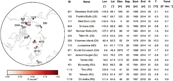
Figure 1. Spatial distribution of the considered boreholes. The colour coding refers to the observed trend expressed as temperature change per decade. The table contains the following key characteristics of the boreholes: ID: data-base ID of the Global Terrestrial Network of Permafrost (GTN-P), Name: name of the borehole (including ISO country code). Lon: longitude in decimal degrees. Lat.: latitude in decimal degrees. Elev.: elevation in meters above sea level. Dep.: depth of the measurement in meters. Start: first year with observations. End: last year with observations. N: total number of years with observations. T: mean temperature in °C of all available years. Trend: trend in °C change per 10 years.
Download figure:
Standard image High-resolution image2.2. ESM simulations
We consider ground temperature time series stemming from ESM simulations. ESMs aim at capturing major aspects of Earth system dynamics by simulating ocean, atmosphere, and land systems in a coupled fashion. Land modules typically solve the water and energy balance and account also for cryosphere processes like snow dynamics. In ESMs, soils are represented through a stack of layers that can store and exchange energy and water and thus can simulate the thermal state of the sub-surface. For this study, ESM simulations contributing to the sixth phase of the Coupled Model Intercomparison Project (CMIP6) (Eyring et al 2016) are used. Long simulations driven with constant pre-industrial radiative forcing (PIC) are used to characterize internal climate variability without human influence (Eyring et al 2016). In a detection and attribution setup, these simulations can be used to assess how likely an observed change might have occurred due to internal climate variability alone. HIST simulations consider the effect of human emissions (greenhouse gases, aerosols) on the climate system throughout the past century until 2014 (Eyring et al 2016). In addition, HIST simulations also account for natural variations in solar forcing and the effect of large volcanic eruptions. These simulations can be used to assess if an observed change is captured by ESMs driven with all relevant forcings. HIST natural (HIST-NAT) simulations are similar to HIST simulations but only account for variations in solar forcing and large volcanic eruptions throughout the past century (Gillett et al 2016). HIST-NAT simulations are used to investigate if naturally occurring variations in the radiative forcing are sufficient to capture observed trends using ESM simulations.
All CMIP6 data are prepared through a centralized pre-processing (Brunner et al 2020) that ensures consistency of the data and includes the interpolation of the model outputs to a common 2.5° grid. For HIST and HIST-NAT simulations, only data covering the time window of the observations are considered. The long PIC simulations are split into non-overlapping 37 year segments, each mimicking the observed period as if it could have occurred under pre-industrial conditions and with no variations in natural radiative forcing. Supplementary table S1 lists the considered models together with the number of available runs (HIST and HIST-NAT) or the number of available segments (PIC). In total, 659 (PIC), 500 (HIST), and 116 (HIST-NAT) samples are available for the considered experiments. Supplementary table S1 also lists the depth as well as the number of layers for each model.
2.3. Linking observations and ESM simulations
ESM simulations are compared to borehole data as follows. First only the grid-cells that contain boreholes are selected. Subsequently, years lacking observations are set to missing for each grid-cell individually. Due to differences in how ESMs represent shorelines in coarse grids, the number of available simulations can be reduced for boreholes in coastal regions. Supplementary table S2 lists the number of ESM simulations available at each borehole for all considered experiments. At each of these grid-cells, the soil-layer with the depth closest to the depth of observation is used. Since not all models cover the depth of observations, a sub-set of simulations with soil depths consistent with the depth of observations is also considered. See supplementary table S2 for the resulting number of simulations for each borehole and all experiments. Note also that no simulations from the HIST-NAT experiments are available for the borehole Janssonhaugen, Svalbard (Isaksen et al 2007) in the reduced ensemble.
Figure 2 shows the pre-processed time series of observed and simulated temperature anomalies at 17 m depth in rock glacier Murtèl-Corvatsch in the Swiss Alps, operated by the Swiss Permafrost Monitoring Network PERMOS (Permos 2021b). The time series are cantered to have a zero mean and years missing in the observed record are also set to zero in the simulations. Note also that the 10th to 90th percentile range of the model simulations is shown instead of individual runs to aid visualization. Data from all other boreholes are shown in supplementary figure S1 (all simulations) and figure S2 (simulations with depths that cover the depth of the observation).
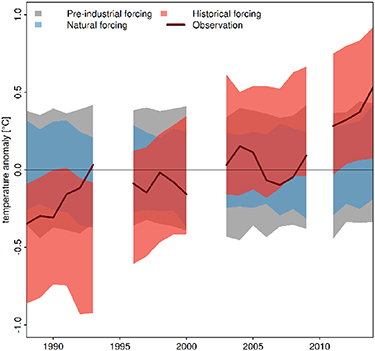
Figure 2. Observed and simulated ground temperature anomalies at Murtèl-Corvatsch in Switzerland. Solid line: observation at 17 m depth. Shaded areas: 10th to 90th percentile of available model simulations belonging to pre-industrial, historical natural and historical simulations. Note that the simulations are masked to match observed temporal coverage.
Download figure:
Standard image High-resolution image3. Methods
3.1. Estimating trends
Change in observed and simulated ground temperature is quantified using linear trends in time estimated by ordinary linear regression at each location. Trends are expressed in units of °C change per decade (i.e. 10 years). Subsequently the mean trend over all locations is computed. This procedure results in one northern hemisphere mean trend estimate for the observations and each simulation experiment.
3.2. Detection and attribution of anthropogenic climate change
Here we follow the abovementioned definition of climate change detection and attribution (Hegerl et al 2006) and evaluate the observed trend in the context of ESM simulation experiments with PIC, HIST and HIST-NAT radiative forcing. For each CMIP6 simulation experiment, we exploit the large number of samples available to construct the empirical trend distribution. Climate change detection can be claimed if the observed trend is unlikely given trends implied by the PIC simulations. To claim attribution to human induced climate change the following two conditions have to be fulfilled. First, the observed trend is consistent with (or likely given) the HIST simulations. Second, the observed trend is inconsistent with trends implied by HIST-NAT simulations. In other words, attribution can be claimed if the considered models only reproduce the observed trend if human influence on the climate system is considered.
The likelihood of the observed trend given the simulation experiments is quantified using approximate p-values defined as the fraction of simulated trends that are smaller than the observed trend. Very large or small values indicate that the observed trend is unlikely given the considered simulation experiment. In particular, large p-values suggest that the observed trend is larger than the expected trends. Here we follow the calibrated language of the intergovernmental panel on climate change (IPCC) (Chen et al
2021) and use p > 0.66 to indicate a likely, p > 0.9 to indicate a very likely and p > 0.99 to indicate virtually certain detection. Medium p-values (e.g.  ) indicate consistency between the observed and the simulated change.
4. Results
4.1. Comparing the spread of the full and the reduced model ensemble
We first compare the spread of the full ensemble with the reduced ensemble that only contains models that cover the depth of the observations (supplementary table S3). This shows that the variance of the full ensemble is unanimously larger than the variance of the reduced ensemble. This feature might be related to (a) the smaller sample size of the reduced ensemble or (b) to increased dampening of decadal variability in simulated ground temperature with increasing depth. Irrespective of the reasons for the difference in variance, the assessment of the full ensemble is therefore expected to be more conservative, i.e. it is less likely for observed trends to be located on the tails of the distributions implied by the simulations. To err on the side of caution, the remainder of this paper therefore focuses on the full ensemble. However, all computations are repeated for the reduced ensemble and are presented in the supplement.
4.2. Mean trend over all boreholes
Observed and simulated mean trends across all boreholes are shown in figure 3(a). The mean trend in the observations increases at a rate of approximately 0.4 °C per decade. Mean trends found in PIC and HIST-NAT simulations fluctuate around zero. Moreover, the observed trend is with high certainty (p > 0.99) larger than trends that occur due to internal climate variability and very likely (p > 0.9) larger than trends related to naturally forced climate change (figure 3(b)). In contrast, trends of the HIST simulations clearly encompass the observed value. This shows that the observed mean trend can only be explained by ESM simulations that are driven with HIST radiative forcing that considers human emissions. In summary, the analysis presented in figure 3 shows that observed permafrost temperatures in the considered boreholes contain a detectable climate change signal (inconsistent with PIC) that can be attributed to anthropogenic climate change (consistency with HIST and inconsistency with HIST-NAT). A supplementary analysis that is based on the reduced ensemble confirms this result (supplementary figure S3).
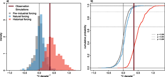
Figure 3. Observed and simulated mean trends in permafrost temperatures across all stations. (a) Histograms of mean trends from pre-industrial, historical natural and historical climate model simulations. The vertical line indicates the global mean of the observed trends. (b) Empirical distribution functions of the trends from the considered climate model simulations alongside the observed mean trend. Horizontal lines indicate approximate p-values considered for this study.
Download figure:
Standard image High-resolution image4.3. Trends from individual boreholes
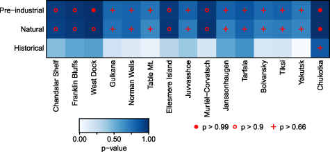
Given the significant results derived from the mean trend across all boreholes, we also investigate the likelihood of the observed trends at individual locations given the PIC, HIST-NAT, and HIST simulations. Figure 4 shows p-values of the observed trends at all locations for each simulation experiment. Despite the poor signal-to-noise ratio expected for the analysis of individual boreholes, p-values derived from the PIC and HIST-NAT simulations always exceed p > 0.66 and at six boreholes p > 0.9 or p > 0.99. This shows that observed trends in ground temperatures at all boreholes are at least likely larger than trends expected due to internal climate variability or naturally forced climate change alone. Moreover, at most boreholes, the observed trends are consistent with the HIST simulations that account for human influence on the climate system. Note that in some cases, very low p-values indicate that trends derived from HIST simulations can systematically exceed the observed trends. The latter result can be directly related to observed and simulated time series for which the simulated warming of HIST is smaller than the observed increase in temperature at the respective locations (supplementary figure S1).
Figure 4. Approximate p-values of the observed trends given the pre-industrial, historical-natural and historical simulation experiments. Large p-values indicate that the observed trend is larger than what is expected given the simulations. Intermediate values suggest that the observed trend is consistent with the simulations.
Download figure:
Standard image High-resolution image
Results based on the analysis of the reduced ensemble that only considers models that reach down to the depth of the observations is generally consistent with the results derived from the full ensemble (supplementary figure S4). Nonetheless, some differences are noted. For the PIC experiments, the approximate p-values of the reduced ensemble are generally larger (p < 0.9 in 10 of 15 cases), indicating a higher confidence in the detection of a systematic trend at the borehole scale. This, in turn, is consistent with the lower spread of the reduced ensemble (see supplementary table S3). Similar behaviour is found at most boreholes for the analysis of HIST-NAT. However, the latter result needs to be interpreted with caution since the reduced ensemble for HIST-NAT only has nine members at most locations, implying highly uncertain approximate p-values. Interestingly, the analysis of the HIST simulations of the reduced ensemble results in large approximate p-values (p > 0.66 and p > 0.9) at six locations. This implies that for these boreholes, the observed trends are significantly larger than the trends of the HIST simulations in the constrained ensemble. In these cases, a careful inspection of the associated time series (supplementary figure S2) shows that the HIST simulations do exhibit a trend but underestimate the observed warming.
5. Discussion
The scope of this investigation is to assess the likelihood of observed trends in permafrost temperatures given simulations that account for natural and human influence on the climate system within the climate change detection and attribution framework (Hegerl et al 2006). To this end, permafrost temperature trends from selected long-term in-situ measurements are compared to empirical trend distributions derived from large ensembles of ESM simulations driven with pre-industrial, HIST-NAT, and HIST radiative forcing. Thus, the analysis combined evidence from observations and ESMs using an empirical approach facilitated by many available samples for each of the considered simulation experiments.
We note that the empirical approach to climate change detection and attribution makes the analysis potentially sensitive to the finite sample of simulations used to estimate distributions. Furthermore, the choice to consider the ensemble of opportunity within the CMIP6 archive puts more weight on models with more initial condition ensemble members or longer pre-industrial control simulations. However, theoretically more sophisticated approaches for climate change detection and attribution make strong assumptions regarding the underlying statistical model, typically including the normality of residuals as well as additivity of forced response and internal climate variability (Allen and Stott 2003, Ribes et al 2016). While such assumptions are often meaningful and required for enhancing the signal-to-noise ratio, the resulting methods add complexity and uncertainty to the analysis. The presented study, in turn, takes full advantage of the abundance of ESM integrations to empirically approximate the distributions of permafrost trends given different radiative forcing.
We also note uncertainties related to simplified modelling assumptions, which are necessary when simulating thermal properties of soils in ESMs at the global scale. For example, there is a scale mismatch between boreholes and the resolution of the models. Moreover, models differ significantly in the maximum ground depth and the number of considered soil layers. In addition, imperfect model physics and un-resolved processes may cause model errors. Moreover, ESM temperatures can be biased leading to differences in absolute values compared to observations. Finally, not all considered ESMs reach down to the depth of the observations.
Besides model uncertainties, limits of the observational record must be considered for a balanced assessment of the evidence. Most importantly, only boreholes compiled by Biskaborn et al (2019) that are publicly available (GTN-P 2021) were used to ensure reproducibility. Furthermore, the availability of climate model simulations implied that only observations until 2014 were used, which further reduces the likelihood of discriminating systematic trends against internal climate variability. In addition, point-scale ground temperature observations are considerably influenced by natural environmental (e.g. ground characteristics and surface cover) and climate variability (e.g. small-scale variations in air temperature and precipitation), which can obscure underlying climate change signals.
To alleviate these issues the following measures for enhancing the signal to noise ratio were taken: first, focussing on permafrost temperatures at DZAA was a guiding feature when designing the analysis. At DZAA, permafrost temperatures have negligible intra-annual and reduced year-to-year variability compared to surface temperatures. Therefore, they are less influenced by short-term climatic fluctuations. Second, the analysis focussed on comparing long-term trends, which are driven by overarching shifts in climatic conditions. Third, the primary analysis of this paper focused on the mean trend across all boreholes which reduced effects of natural spatial variability and hence further increased the signal to noise ratio. In addition, a supplementary analysis confirmed the validity of the results when only considering ESMs with soil depths that are consistent with the observations.
6. Conclusions
In conclusion the analysis supports a high degree of confidence in the finding that the observed mean trend in permafrost temperature across all boreholes is inconsistent with internal climate variability and that that ESM simulations only capture the observed mean trend if human influence on the climate system is considered. In addition, a secondary analysis finds an influence of anthropogenic global warming on permafrost temperature at the borehole scale. Despite the reduced statistical confidence this is remarkable, since detecting and attributing climate change at individual locations is generally considered to be hampered by large degrees of environmental and climate variability (Zwiers and Zhang 2003, Stott et al 2010).
Although the results provide considerable evidence in support of the hypothesis that human influence on the climate system is driving observed permafrost temperature warming, we note that the results only represent what is possible with the latest generation of ESMs and the considered observations. Therefore, the findings should not be interpreted in isolation. Here it is essential to recall that the presented research is fully consistent with current understanding of impacts of anthropogenic climate change on permafrost (IPCC 2019, Burke et al 2020, Guo et al 2020). Nonetheless, a strong need for continuous and global efforts to observe and share permafrost temperature remains to monitor climate change impacts and to foster climate adaptation in environments with amplified warming rates such as the Arctic and Mountain regions.
In summary, this study shows that the mean permafrost temperature trend across 15 boreholes around the northern hemisphere can only be explained by ESM simulations, if effects of human emissions on the climate system are considered and that systematic climate change patterns are emerging at the borehole scale. Consequently, the combined analysis of spatial mean trends across locations and the assessment of individual boreholes supports the hypothesis that observed permafrost warming can be attributed to anthropogenic climate change.
Acknowledgments
Climate model simulations stem from the sixth phase of the Coupled Model Intercomparison Project (CMIP6) and are available through the Earth system grid federation (https://esgf-node.llnl.gov/projects/cmip6/). We acknowledge CMIP6 data processing by Urs Beyerle, Lukas Brunner, and Ruth Lorenz. Annual mean permafrost observations were previously assembled by Biskaborn et al (2019) and are available for download at https://doi.pangaea.de/10.1594/PANGAEA.930669. Note that some of the meta-data of the time series are erogenous. The correct meta-data can be accessed through http://gtnpdatabase.org/boreholes/xyz where xyz indicates the GTN-P ID. We are indebted to all persons and institutions who have contributed to long-term permafrost temperature observations.
Funding
A G was supported by the German Federal Ministry of Education and Research (BMBF) and the European Research Area for Climate Services ERA4CS with funding reference 518 Number 01LS1711C (ISIPedia project). L G was partially supported by the European Union's Horizon 2020 research and innovation programme under grant agreement No. 101003687 (PROVIDE Project).
Supplementary data (0.8 MB PDF)