Snow Depth and Air Temperature Seasonality on Sea Ice Derived From Snow Buoy Measurements
 Marcel Nicolaus*
  Mario Hoppmann
  Stefanie Arndt
  Stefan Hendricks
  Christian Katlein
  Anja Nicolaus
  Leonard Rossmann
  Martin Schiller
  Sandra Schwegmann
- Alfred-Wegener-Institut Helmholtz-Zentrum für Polar- und Meeresforschung, Bremerhaven, Germany
Snow depth on sea ice is an essential state variable of the polar climate system and yet one of the least known and most difficult to characterize parameters of the Arctic and Antarctic sea ice systems. Here, we present a new type of autonomous platform to measure snow depth, air temperature, and barometric pressure on drifting Arctic and Antarctic sea ice. “Snow Buoys” are designed to withstand the harshest environmental conditions and to deliver high and consistent data quality with minimal impact on the surface. Our current dataset consists of 79 time series (47 Arctic, 32 Antarctic) since 2013, many of which cover entire seasonal cycles and with individual observation periods of up to 3 years. In addition to a detailed introduction of the platform itself, we describe the processing of the publicly available (near real time) data and discuss limitations. First scientific results reveal characteristic regional differences in the annual cycle of snow depth: in the Weddell Sea, annual net snow accumulation ranged from 0.2 to 0.9 m (mean 0.34 m) with some regions accumulating snow in all months. On Arctic sea ice, the seasonal cycle was more pronounced, showing accumulation from synoptic events mostly between August and April and maxima in autumn. Strongest ablation was observed in June and July, and consistently the entire snow cover melted during summer. Arctic air temperature measurements revealed several above-freezing temperature events in winter that likely impacted snow stratigraphy and thus preconditioned the subsequent spring snow cover. The ongoing Snow Buoy program will be the basis of many future studies and is expected to significantly advance our understanding of snow on sea ice, also providing invaluable in situ validation data for numerical simulations and remote sensing techniques.
Introduction
The sea ice cover of the polar oceans plays a dominant role in the Earth’s climate system, and at the same time, its evolution is a direct indicator of global changes. Most Arctic and Antarctic sea ice is covered with snow most of the year (Warren et al., 1999; Massom et al., 2001). The presence of this snow cover on the surface alters the properties of the underlying sea ice and the associated physical and biological processes as well as biogeochemical fluxes across the atmosphere-ice-ocean interfaces through a number of direct and indirect effects (e.g., Sturm and Massom, 2009). In addition, snow on sea ice contributes to the entrainment and transport of contaminants such as soot (Grenfell et al., 2002) and mercury (Jacobi et al., 2012; Steffen et al., 2014), it impacts travel and hunting conditions during subsistence activities (Gearheard et al., 2006), and reduces the efficiency of icebreakers. While detailed reviews of the role of snow on sea ice and its challenges are given by Massom et al., 2001 and more recently by Webster et al. (2018), we here summarize the most important aspects with regard to the presented instrument and dataset.
Due to its exceptional insulative properties and its own mass, snow plays a governing role in sea ice thermodynamics, and consequently determines its mass balance to a great extent. In particular it contributes to snow ice and superimposed ice formation and thus sea ice thickening from the top (Worby et al., 1998; Haas et al., 2001; Willmes et al., 2006; Nicolaus et al., 2009; Arndt et al., 2017). This thickening is mainly observed across large areas of the Southern Ocean, but is also expected to be more important in a future thinner Arctic sea ice regime (Granskog et al., 2017). In addition to these direct effects, snow also complicates the interpretation and retrieval of sea ice geophysical parameters, such as sea ice thickness and volume, from in situ and remote sensing methods. Retrievals from upward-looking sonar data require accurate assumptions of snow depth and -densities to convert from draft into sea ice thickness (Behrendt et al., 2015). Laser altimetry from satellites detects snow freeboard and is thus dependent on accurate assumptions about the snow cover to convert these freeboard measurements into sea ice thickness (Kwok et al., 2004). Similarly, for the current radar (CryoSat-2, Sentinel-3A/B, AltiKa) altimeter missions, the interface and volume snow radar backscatter has a notable impact on the radar ranging in the freeboard retrieval process (Kurtz et al., 2014; Kwok, 2014; Ricker et al., 2015; Nandan et al., 2017; King et al., 2018).
Antarctic sea ice in particular exhibits a comparably high snow load to ice thickness ratio (Worby et al., 2008), resulting in a strong impact of the freeboard. An accurate estimation of snow depth is therefore especially sensitive to the freeboard to thickness conversion (Kwok and Cunningham, 2008; Schwegmann et al., 2016). The sea-ice thickness retrieval processing chain in the past usually relied on a monthly climatology of snow depth and density (Warren et al., 1999) typically modified for different ice types (e.g., Webster et al., 2014) to reflect for interannual variability. In the Southern Hemisphere, information on snow depth on sea ice can be derived from passive microwave data or parametrized from laser altimetry (Kern and Ozsoy-Cicek, 2016). However, significant uncertainties remain in remote sensing of snow depth in the past, which only may be resolved with a new generation of dedicated sensors or sensor combinations (CryoSat-2/ICESat-2) or the planned Copernicus Polar Ice and Snow Topography Altimeter (CRISTAL) (Kern et al., 2020). The combination of radar altimeters with different wavelength, e.g., Ku and Ka-Band altimeters, as well as the combination of radar and laser altimeters are currently the most promising candidates to observe basin scale snow depth on sea ice with satellite remote sensing (Armitage and Ridout, 2015; Guerreiro et al., 2016; Lawrence et al., 2018; Kwok et al., 2020).
At present, the availability of snow depth observations on Arctic and Antarctic sea ice remains sparse, especially when considering that snow accumulation and redistribution are highly variable on small spatial and temporal scales (e.g., Sturm et al., 2002; Webster et al., 2014). Even the precipitation processes and distribution are still highly uncertain and a major research topic (e.g., Webster et al., 2018; Boisvert et al., 2020). As a consequence, the representation of the snow pack in numerical models is a major challenge, e.g., with respect to the number of layers in the model (Lecomte et al., 2011; Liston et al., 2018), the distribution of snow into different ice thickness (Castro-Morales et al., 2014) or the role of snow cover effects on sub-grid scales (Abraham et al., 2015).
Multi-seasonal drifting experiments such as SHEBA (1997/98), the Russian North Pole Stations (since 1937), the drift of TARA (2006/07), and the Norwegian young sea-ice experiment (N-ICE, 2015) have been exceptionally useful in understanding the general seasonal evolution of surface properties in the Arctic (e.g., Sturm et al., 2002; Nicolaus et al., 2010; Sankelo et al., 2010; Granskog et al., 2016; Merkouriadi et al., 2017). The MOSAiC program in 2019/20 was the most comprehensive program ever to better understand the snow cover on sea ice and its interaction with the ice and the atmosphere (Krumpen et al., 2020). Some measurements of summer snow depth on Arctic sea ice are even available from adventurers (Gerland and Haas, 2011). Since similar multi-seasonal experiments are much more challenging to collect in the Antarctic in terms of logistics, comparable year-round datasets or even climatology are entirely lacking, with only sporadic compilations being available from the literature (Massom et al., 2001), from single ship-borne field campaigns (e.g., Haas et al., 2008; Nicolaus et al., 2009; Willmes et al., 2009; Toyota et al., 2016), from ASPeCT bridge observations (Worby et al., 2008; Ozsoy-Cicek et al., 2011) or from monitoring activities on landfast sea ice near manned stations (Heil, 2006; Lei et al., 2010; Hoppmann et al., 2015). One of the few winter snow data sets from Antarctica is presented by Arndt and Paul (2018), highlighting the importance to distinguish the age and type of the underlying sea ice to derive snow properties on large scales.
Additional time series of snow depth on sea ice are available over the last two decades from autonomous platforms drifting on sea ice. Depending on the platform, snow depth may either be derived from ultrasonic range finders as on Automatic Weather Stations (AWS) or Ice Mass-balance Buoys (IMB) (Richter-Menge et al., 2006) or thermistor strings (Jackson et al., 2013). But these direct observations are still too few to enable the compilation of large-scale seasonal snow depth data sets. Better regional coverage during Arctic spring has been achieved with airborne wide-band radar measurements by the NASA Operation IceBridge (Kurtz and Farrell, 2011; Webster et al., 2018).
In order to ease and increase the acquisition of snow observations, we developed a new kind of simple to deploy and affordable autonomous platform, which we refer to as “Snow Buoy.” In this study, we present a unique and growing dataset of snow depth and air temperature time series measurements on Arctic and Antarctic sea ice, recorded by these Snow Buoys. We present and discuss the concept and technical details of this new buoy type, including the description of data processing and accessibility, and conduct comparisons of the buoy data to internationally well-regarded baseline measurements. Over the last years, 79 Snow Buoys were deployed either on drifting pack ice or on landfast sea ice. Highlights presented in this study are results from two sets of buoys deployed in the Weddell Sea (Antarctica) and three sets of buoys in the central Arctic Ocean. The corresponding data sets are collectively analyzed in space and time, allowing to derive monthly accumulation and ablation estimates and their regional differences. Finally, we discuss the advantages, challenges, and limitations associated with these autonomous measurements.
Methods: Snow Buoy Description
Snow Buoys
Snow Buoys are simple and affordable platforms to obtain observations of snow depth on Arctic and Antarctic sea ice. Their development was based on the need for more in situ observations that cover the entire annual cycle and help to characterize the seasonality of snow depth in different regions. Snow Buoys also observe near surface air temperature and barometric pressure. These data are reported in near real time (NRT) to the Global Telecommunication System (GTS), using a World Meteorological Organization (WMO) unique identifier (since 2015, see Supplementary Table 1). In this way, the buoys contribute to various international efforts aiming to improve numerical weather forecasts in the high- and mid-latitudes, by increasing the number of observations in the polar oceans. Snow Buoys were developed as a cooperation between the Alfred-Wegener-Institut Helmholtz-Zentrum für Polar- und Meeresforschung (Bremerhaven, Germany) and the manufacturer MetOcean Telematics (Halifax, Canada).
The 2.55 m tall Snow Buoy consists of two parts, (1) a 0.8 m high and 0.25 m diameter main body carrying the electronics and batteries, and (2) a 1.75 m high mast, carrying a frame with four ultrasonic sensors at 1.5 m above the main body, and on top the air temperature sensor and the Iridium and GPS antennas (Figure 1). A surface temperature sensor and a barometer are integrated into the main body. The hull, mast, and sonar supports are made from 6061-T6 aluminum. A white wooden ablation shield (not shown in the figure) supports the beacon on the ice surface and reduces ice ablation at the installation site. Snow Buoys have no flotation unit in order to keep them small and the surface impact minimal. The weight of the buoy is approx. 40 kg, depending on the battery configuration. Power supply is realized by Lithium (14.6 V) or Alkaline (17.0 V) batteries (cells). Although Lithium batteries provide a more reliable and long-lasting power supply in particular during polar winters, 42 of 79 units have been deployed with Alkaline batteries. Reasons are logistical (regulations on the transport of dangerous goods) and environmental issues. Both battery types guarantee operation times longer than 1 year (Supplementary Figure 1 and Table 1).
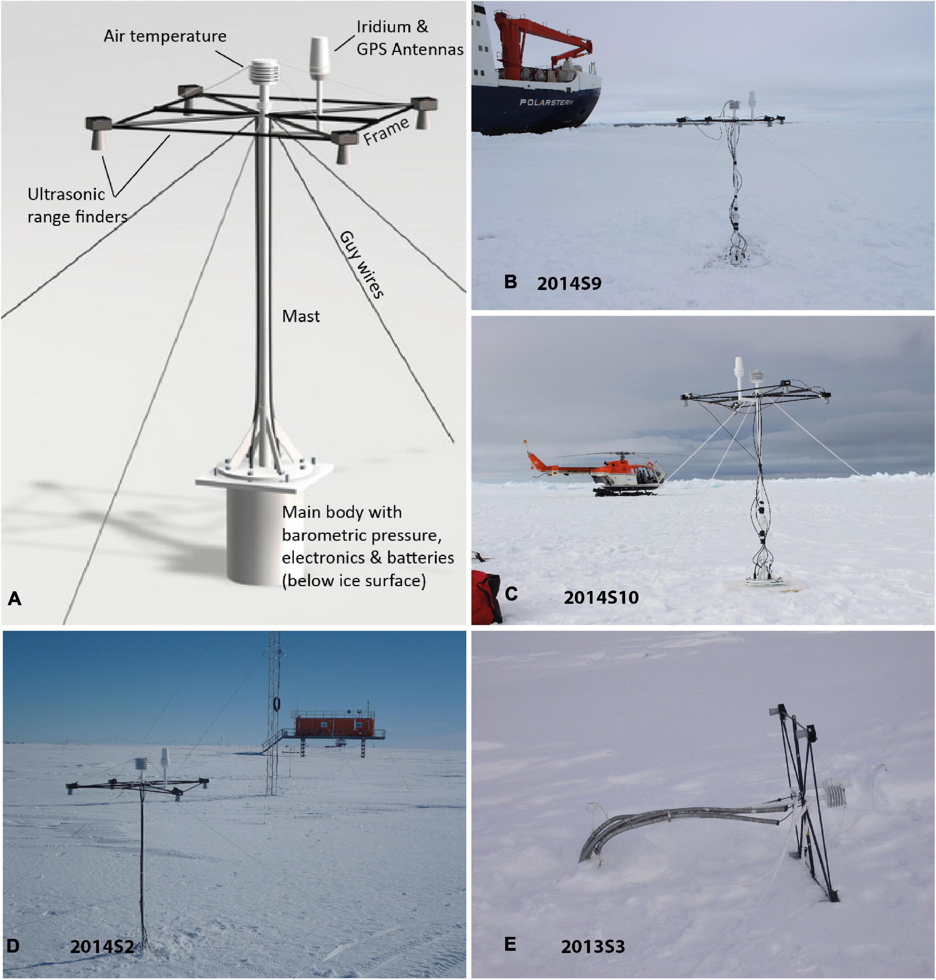
Figure 1. (A) 3-dimensional sketch of a Snow Buoy with annotated sensors. An ablation shield (approx. 1 × 1 m) is installed directly under the top plate of the main body during deployment, but this is not shown here. (B–E) Photographs of Snow Buoys after deployment: 2014S9 and 2014S10 were deployed on sea ice in the Weddell Sea in January 2014. 2014S2 was deployed on the ice shelf close to Neumayer III station (the trace gas observatory is the orange container in the back). 2103S3 after it fell over on the fast ice of Barrow, Alaska, and it was modified with metal hoses to protect against polar foxes.
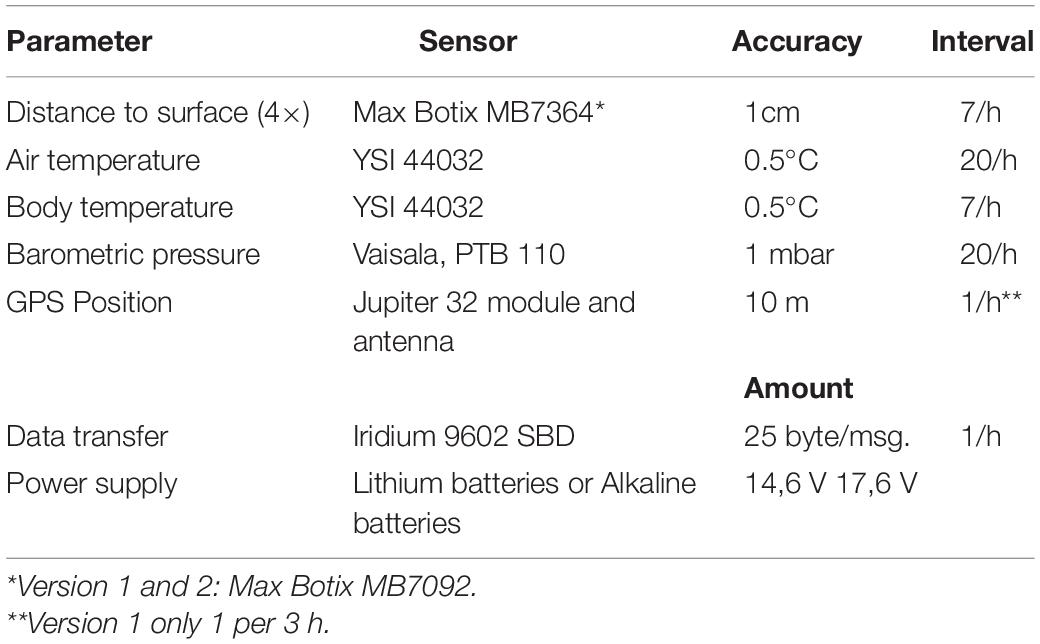
Table 1. Overview of sensors and measurement intervals as used in Snow Buoys Version 3.
The distance to the surface is measured with four ultrasonic range finders MB7364 (Max Botix, Brainerd, MN, United States) in hourly intervals. The four-sensor concept provides redundancy in case of single sensor failures and increases data quality, but also allows more insights into small-scale snow variability in the vicinity of the buoy. The sensors use a narrow beam for surface detection, such that the signal is mostly returned from an area of max. 0.3 m diameter right under the sensor. This sensor was selected based on experience in long-term autonomous applications in snow depth measurements by the Swiss mountain and avalanche surveillance stations. The first version (five prototypes, 2013S1 to 2013S5) used the older MB7052 without internal temperature correction. For these buoys, an additional temperature correction was performed based on the measured air temperature. Snow depth results from relative measurements of surface height changes (distance from the ultrasonic sensor) and absolute measurements under each sensor during deployment. In some cases, these initial measurements were not performed or not meaningful (e.g., on the ice shelf). Then, only relative changes of snow depth can be derived, assuming an initial snow depth of 0.00 m.
It has to be emphasized at this point that Snow Buoys measure a “change in surface height relative to the original ice surface” rather than the actual “snow depth.” “Surface height” is usually impacted by freeboard changes as a function of sea ice melt/formation, density and snow mass, whereas “snow depth” may be impacted by snow metamorphism, e.g., superimposed ice or snow ice formation. However, since “snow depth,” is a much more common term in particular in connection to most related discussions on snow energy and mass balance, we decided to use this term in our description and discussion of most Snow Buoy data, but to still label the original measurements (time series data) as “surface height”. This terminology has to be considered especially when comparing data from this study and method to other observational techniques or numerical simulations.
Air temperature is measured by a YSI 44032 thermistor (YSI, Yellow Springs, OH, United States), mounted in a radiation shield to reduce the effect of solar heat absorption. The buoy does not carry sufficient power to enable instrument ventilation. The sensor provides an accuracy of ±0.5°C, but this does not include uncertainties (warming) by absorption of solar short-wave radiation. Buoy body temperature is also measured by a YSI 44032 thermistor. The sensor is mounted within the main body in approx. 0.6 m depth, providing an internal temperature similar to that of the surrounding sea ice. Barometric pressure is measured by a PTB110 barometer (PTB, Braunschweig, Germany), which is mounted in the upper surface part of the main body. Geographic position is measured with a Jupiter 32 GPS module (Navman, Gladesville, NSW, Australia). All sensor specifications and standard measurement intervals are summarized in Table 1. Data transmission is provided by an Iridium 9602 module with external antenna, using the Short Burst Data (SBD) protocol. A single submitted data set, containing all measurements plus some additional control and status variables is 25 bytes. Given the standard configuration of measurement intervals (Table 1) and hourly reporting, the monthly data volume amounts to approx. 18 kb. The hourly messages are immediately transferred to the GTS.
Based on the experience over the years, where various data quality issues arose, a number of hardware improvements were realized. Early units sometimes experienced electronic failures after strong snow drift, and additional internal connections to ground the electronics were made to reduce these electrostatic discharge problems. Drifting snow is still an issue in terms of data quality (see below), but has not caused failures of the entire unit since this change. Additionally, between Versions 1 and 2, an internal controller was replaced with a more reliable and robust one. Other improvements included strengthening of the detachable mast, and the guy wiring. Installations in Barrow, Alaska, were equipped with optional cable protection against polar foxes (Figure 1E).
The overall design allows a quick and straightforward deployment mostly independent of deployment logistics and may even be performed by one or two persons with very little training within 30 min. Snow Buoys were mostly installed on level sea ice, with snow and ice conditions representative of the surrounding area (Figure 1). They have been deployed by various means: during ice stations from icebreakers with direct access to the ice, by helicopter or fixed wing aircraft landing on sea ice, and by snow mobile from a nearby station. For deployment, the initial snow cover is removed in the footprint of the ablation shield and a 0.25 m (10”) diameter, 0.8 m deep hole is carefully drilled into the ice. The hole is then covered by the ablation shield, through which the main body is lowered into the hole. The mast is then fortified against wind using four guy wires anchored to the ice. Finally, the snow surface is restored as much as possible to reduce the impact of the installation to a minimum. Finally, the mast of the buoy and the four guy wires are the only surface obstacles, while all electronics are buried in the ice. This minimizes the effect of the buoy on snow accumulation and re-distribution. After installation, several manual snow depth measurements are performed directly below each ultrasonic sensor to enable conversion to absolute snow depth values during data processing.
Data Concept, Processing, and Quality Control
An essential part of the Snow Buoy concept is a standardized processing and data flow, with the aim to collect data from all Snow Buoys in one common data portal and archiving system. For this, all Snow Buoy data are currently hosted on www.meereisportal.de (or data.seaiceportal.de), a shared data portal and archiving system (Grosfeld et al., 2015). This portal also provides comprehensive metadata and deployment information for all buoys. It also defines a common naming for all Snow Buoys, which is consistent with other buoys of the portal: (1) year of deployment (4 digits), (2) “S” for Snow Buoy (1 character), and (3) counter over all buoys (variable digits): e.g., 2013S2 is the second (over all) Snow Buoy and was deployed in 2013. Internally, the unique International Mobile Equipment Identity (IMEI) number is used as an identifier and allows cross links to any other possible data source or publication when no or even another name is used (Moore, 2016; Itkin et al., 2017). Using the IMEI number as buoy name turned out to be more complicated and creates issues once buoys are re-deployed during different projects/expeditions. After an additional final quality control, all completed time series are published in the data archive and publishing system PANGAEA1, which also provides a digital object identifier (DOI), for each data set (Nicolaus et al., 2017). Since 2015, most Snow Buoys report into the GTS in NRT.
A standard data processing procedure is applied to provide coherent and easily accessible Snow Buoy data to the data portal within 24 h after acquisition. Immediate NRT processing would be possible, but was not requested yet. Since the ultrasonic sensors return directly the distance to the surface, no calibration or conversion work is needed. During processing, five types of filters are applied to the surface height records of each individual sensor in order to flag outliers and invalid data:
• All data before final deployment and after the end of reliable measurements are flagged.
• (only for buoys of Version 1) A linear correction for the dependency of the sound velocity as a function of air temperature is applied for each range measurement.
• A gradient criterium is applied to flag all measurements that exceed a change in surface height of more than 0.1 m/h.
• A 24 h running mean filter flags all measurements that deviate more than 0.03 m from the running mean.
• A buoy specific and manual minimum/maximum filter is applied to support the above-mentioned point-by-point filters.
Note that all filters keep the original measurement and only quality flags are used to mark outliers. This processing does not include any cross-sensor filters or averaging. In a final step, all relative surface height measurements are converted to actual snow depth by assigning the mean value of the initial five range measurements (=5 h) to the in situ snow depth measurement under the respective sensor. This averaging accounts for some variability in the individual distance measurements. Mean snow depth is calculated as the arithmetic mean of all un-flagged measurements at a given time.
Figure 2 shows the time series of Snow Buoy 2014S10, drifting through the Weddell Sea, after standard processing, as available for all buoys from www.meereisportal.de. The four ultrasonic sensors show an increase in surface height from 0.1 m in February 2014 to 1.4 m in May 2016. Colored dots show the filtered data set for each individual sensor and gray dots all measurements that are flagged as outliers (noise). The resulting time series are less noisy and visual plausibility tests are considered sufficient for such a standard processing. Beyond this, individual processing may e.g., remove the low snow depth readings from Sensor 1 (red) in March 2016. Keeping or removing this feature will impact further analysis, e.g., deriving a mean snow depth or interpreting measures of inter-sensor variability. This shows the challenge of consistent and best possible data correction and interpretation. Another interesting feature of this time series is that all four sensors gave unrealistic readings for 2 weeks in June 2014, but continued at the former snow depth range afterward. Reasons for this deviation are rather speculative but could be related to icing of the sensors.
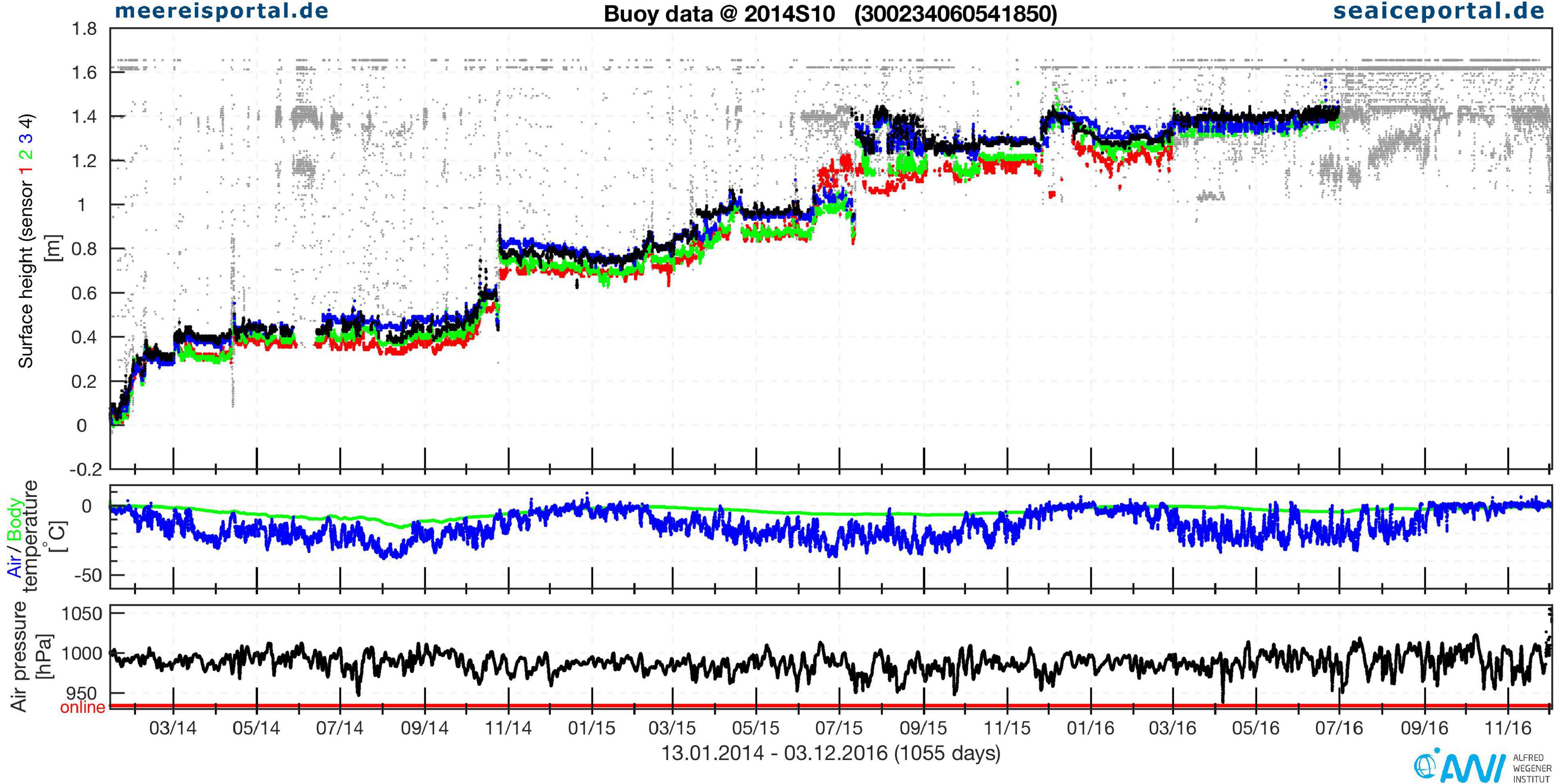
Figure 2. Exemplary plot (standard layout) of Snow Buoy 2014S10, as available from the standard processing on www.meereisportal.de. (top) Surface height from the four sonic sensors. Gray dots represent outliers, which are excluded from the final data product during processing. All surface height measurements after July 01, 2016 were flagged as outliers, because the surface reached close to the sensors. (middle) Air (blue) and body (green) temperature. (bottom) Barometric air pressure (black) and an activity indicator (red line).
Air temperature, barometric pressure, and geographic position are not automatically filtered, but obvious failures of the sensors are flagged manually. For Snow Buoy 2014S10, air temperature and body temperature are shown in the middle panel of Figure 2. Air temperatures below −30°C are found to be typical for several months during winter. Due to the insulating effect of the snow pack, the main body of the buoy remains warmer than −17°C over the entire observation period. During summer, surface melting temperatures are measured. The bottom panel shows the barometric pressure (black line) and an indicator of activity of the buoy (red line).
Results
Snow Buoy Deployments and Technical Performance
In total, 79 Snow Buoys were deployed and operated since January 2013 (Figure 3). Status of the data in this article is from September 15, 2019. 47 units were deployed in the Arctic Ocean, including Snow Buoy 2014S25 on a buoy test site near Barrow, Alaska (Figure 1E). 32 units were deployed in the Weddell Sea, Antarctica, including three on the Ekström Ice Shelf on a test site near the German wintering station Neumayer III (Figure 1D). The test site deployments enabled comparison to baseline data from well-regarded observatories, with easy access of the buoys for potential failure troubleshooting, repair, or other improvements. From the 79 deployments, six individual buoys were redeployed after successful recovery and maintenance (Supplementary Table 1). Details are available from the meta data on www.meereisportal.de.
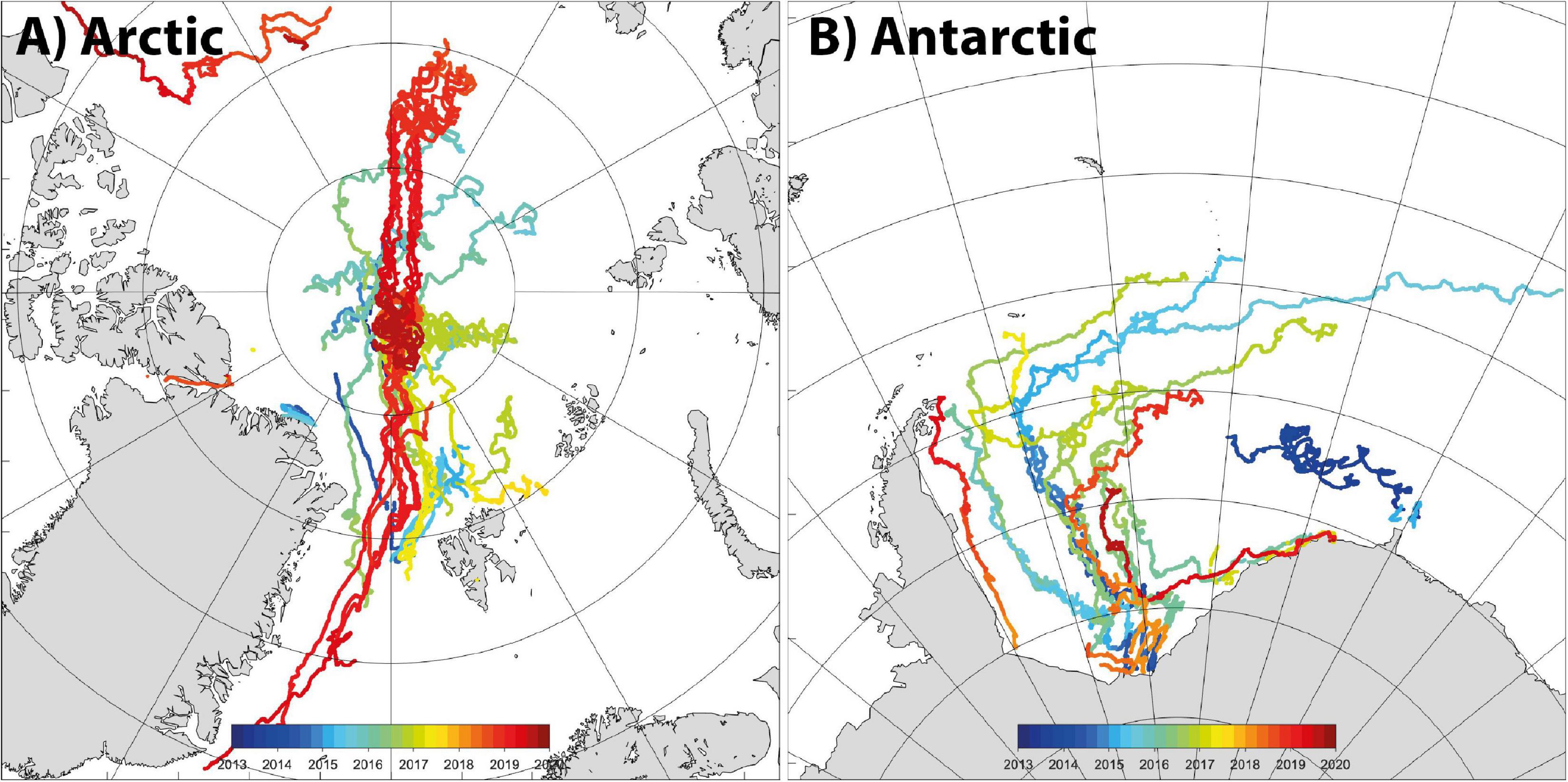
Figure 3. Drift trajectories of all 79 Snow Buoys (A) Arctic and (B) Antarctic. Colors indicate the time of drift (3 months intervals).
The lifetime of an individual buoy depends in most cases on the sea ice conditions and most buoys finally fail in the marginal ice zone, predominantly due to drowning after sea ice melt. Other reasons for failure are destruction through ridging or rafting (e.g., 2017S47) or polar bears that (accidentally) tip over the mast (2013S3). Obvious features for tilting buoys are diverging range measurements of the four sensors or abrupt failures of the entire unit. Buoys were not always deployed for longest possible drifts, but also used in specific regions or for specific research questions, e.g., during the Norwegian new ice experiment N-ICE in 2015 (Itkin et al., 2017). Lifetimes are generally longer in the Weddell Sea (296 days) compared to the Arctic Ocean (200 days, Supplementary Table 1 and Supplementary Figure 1), and mainly depend on the general drift pattern of a given region. Most of the Antarctic buoys were deployed in the eastern or southeastern part of the Weddell Sea in summer during expeditions associated to the resupply of the German Neumayer III station. Their drift trajectory generally followed the clockwise Weddell Gyre circulation (Figure 3b). The measurements of buoys 2014S9, 2014S10, and 2014S12 represent the longest time series of snow depth on drifting Antarctic sea ice so far. Over all, the 24 buoys deployed on Weddell Sea pack ice represent the most comprehensive snow observation datasets in the Antarctic sea ice zone since ISPOL 2004/05 (Hellmer et al., 2008). In the Arctic, most buoys were deployed along the Transpolar Drift during autumn, when research icebreakers usually carry out their central Arctic research missions. In addition to buoys that failed under the conditions described above, few buoys failed due to obvious technical issues. Since the autonomous systems are usually not recovered, error analysis is difficult and the final reason for failure remains mostly speculative. While most internal technical failures may not be analyzed without recovery, the power supply is monitored and transmitted. In general, Lithium cell powered Snow Buoys may expect longer lifetimes, but none of the Snow Buoys on pack ice has ceased operation because of power shortage yet.
Data Quality Assessment and Inter-Comparisons
Although the individual sensors and hardware components have been widely used under alpine and polar conditions before, it is beneficial to perform long-term stability tests and data comparisons with independent instruments. For this purpose, 2013S2 and 2017S54 (Neumayer III) and 2014S25 (Alaska) were installed next to other reference measurements, allowing inter-comparisons with established observatories.
Snow Buoy 2013S2 was installed at the trace gas observatory at the Neumayer III wintering station (Ekström Ice Shelf, Antarctica) from February 2013 to April 2017 (1613 days, Figure 1D and Supplementary Figure 2). Supplementary Figure 2 compares the measurement of the Snow Buoy with the routine measurements of a laser distance sensor mounted on a weather mast (mast shown in Figure 1D, König-Langlo and Raffel, 2017), with more details described in the Supplementary Material. The snow depth evolution at this site was mostly characterized by discrete snow accumulation events during the Antarctic winter (April to November), and periods of no changes or slight compaction and surface melt in Antarctic summer [December to March, see van den Broeke et al. (2009)]. A comparison of both data sets shows that the Snow Buoy time series agrees well with the reference laser measurements, in particular the distinct accumulation events are well reproduced, also under extremely unfavorable conditions and over extraordinary long observational period. Differences were found mainly due to the different foundation of both setups, leading to different settling during summer.
Supplementary Figure 3 shows the comparison of the Snow Buoy 2013S2 data with temperature and barometric pressure data from the Baseline Surface Radiation Network (BSRN) at Neumayer III station (König-Langlo, 2017). The BSRN temperature measurements are performed with ventilated PT-100 sensors. A comparison of both data sets under identical synoptic conditions shows that Snow Buoy air temperatures are consistently higher, with stronger effects at low temperatures. The mean difference between Snow Buoy and BSRN air temperatures was 2.17 ± 1.0°C over the entire period, with 1.41 ± 0.55°C during summer (DJF) and 2.87 ± 1.03°C during winter (JJA). Atmospheric pressure readings agree better over time, and do not show a seasonal difference. Mean difference (Snow Buoy-BSRN) is −0.6 ± 0.7 hPa over the entire time series, which is mainly related to sensor specifications and differences in the measurement height.
Snow Buoy 2014S25 is the second unit that was deployed with the particular aim of inter-comparison measurements. The buoy was installed close to the Earth System Research Laboratory (ESRL) Barrow Observatory in Barrow, Alaska, as part of a buoy-inter-comparison experiment of the International Arctic Buoy Program (IABP). Our analysis reveals similar results as in the case of 2013S2 and the BSRN station on the Antarctic ice shelf. Snow Buoy air temperatures are again consistently overestimated by 1.7 ± 0.9°C, while Snow Buoy barometric pressure matches the ESRL station values quite well (Snow Buoy-BSRN: 0.8 ± 0.3 hPa).
Figure 4 shows the surface height time series of three selected buoys deployed on Arctic and Antarctic sea ice. This example demonstrates outliers and the uncertainties of range measurements. Although this manuscript mainly discusses the mean value of these four readings, some aspects of data quality may be derived directly from the filtering of the measurements of the single sensors: Most outliers are above the real signals, reporting returns from between the snow and the sensor. This is a typical feature and is likely associated with drifting/blowing snow or snowfall events, during which the signal from the snow range finder is scattered back from suspended snow particles, and not from the solid snow surface. In addition, these three examples show that Arctic winter data are generally noisier than data from Antarctic buoys, where noise is almost exclusively related to changes in snow depth. However, Arctic readings often include data with too low snow depth (below the filtered data), a feature that occurs much less in the Antarctic data sets. The Antarctic buoy 2016S38 (Figure 4C) shows some reflections with almost constant offsets, but both features cannot be explained yet. Beyond the outliers, the four snow sensors give mostly coherent readings with respect to temporal changes (Figures 2, 4). Time-invariant offsets between the individual time series mainly result from different initial snow depth, measured under the sensors during deployment.
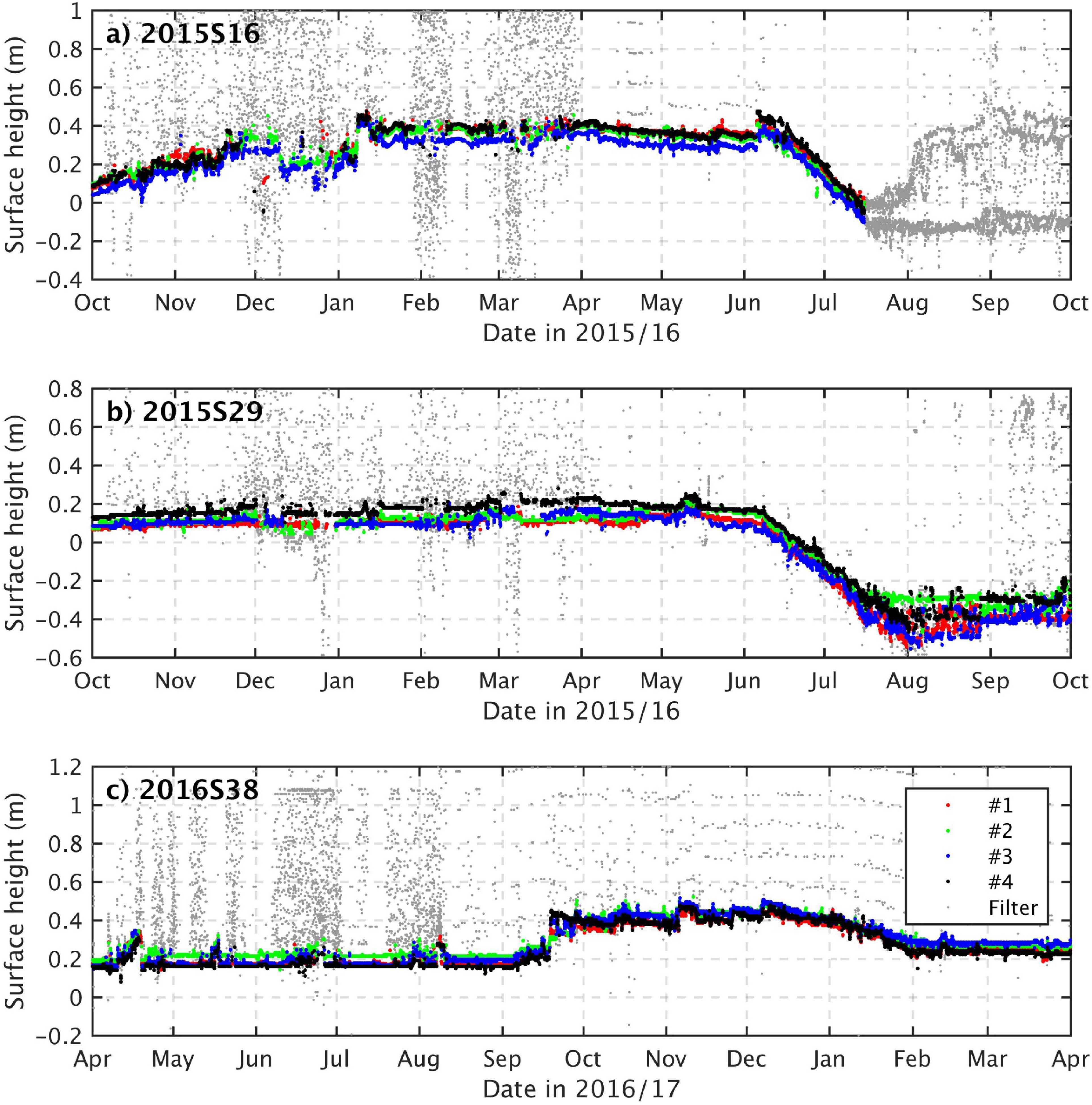
Figure 4. Surface height evolution from three Snow Buoys. Snow Buoys in panels (a,b) were deployed on Arctic sea ice in September 2015, those in panel (c) were deployed on Antarctic sea ice in March 2016. The colored lines show filtered data from each ultrasonic sensor (pinger). Gray dots represent readings, which are excluded from the final data product during processing. All surface height measurements were flagged as outliers once the buoys failed at the end of their lifetime. Drift trajectories of individual buoys are shown in Figure 3 and in more detail in the Supplementary Material.
Snow Depth on Sea Ice in the Weddell Sea
The most remarkable set of snow depth measurements in the Weddell Sea was obtained from the four Snow Buoys 2014S9 to 2014S12, which were installed on medium to large-sized sea ice floes during the Polarstern expedition PS82 in the southeastern Weddell Sea in 2014 (Table 2). All deployment sites consisted of level first-year ice, with sea ice thickness between 1.05 and 1.65 m, and mostly thin snow cover (Figures 1B,C). Figure 5 shows their locations along the drift on different dates together with the sea ice concentration. All buoys completed more than one full annual cycle of measurements (Supplementary Table 1) and finally failed due to disintegration of the ice floe. The disintegration of the corresponding ice areas were confirmed by high-resolution Synthetic Aperture Radar (SAR) images (not shown). Ultimately, 2014S10 reported measurements for almost 3 years (1054 days) and represents the longest time series of all drifting Snow Buoys.
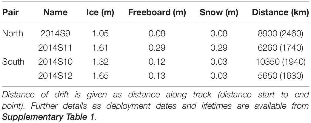
Table 2. Deployment information (sea ice thickness, freeboard, and snow depth) of selected Snow Buoys in the Weddell Sea.
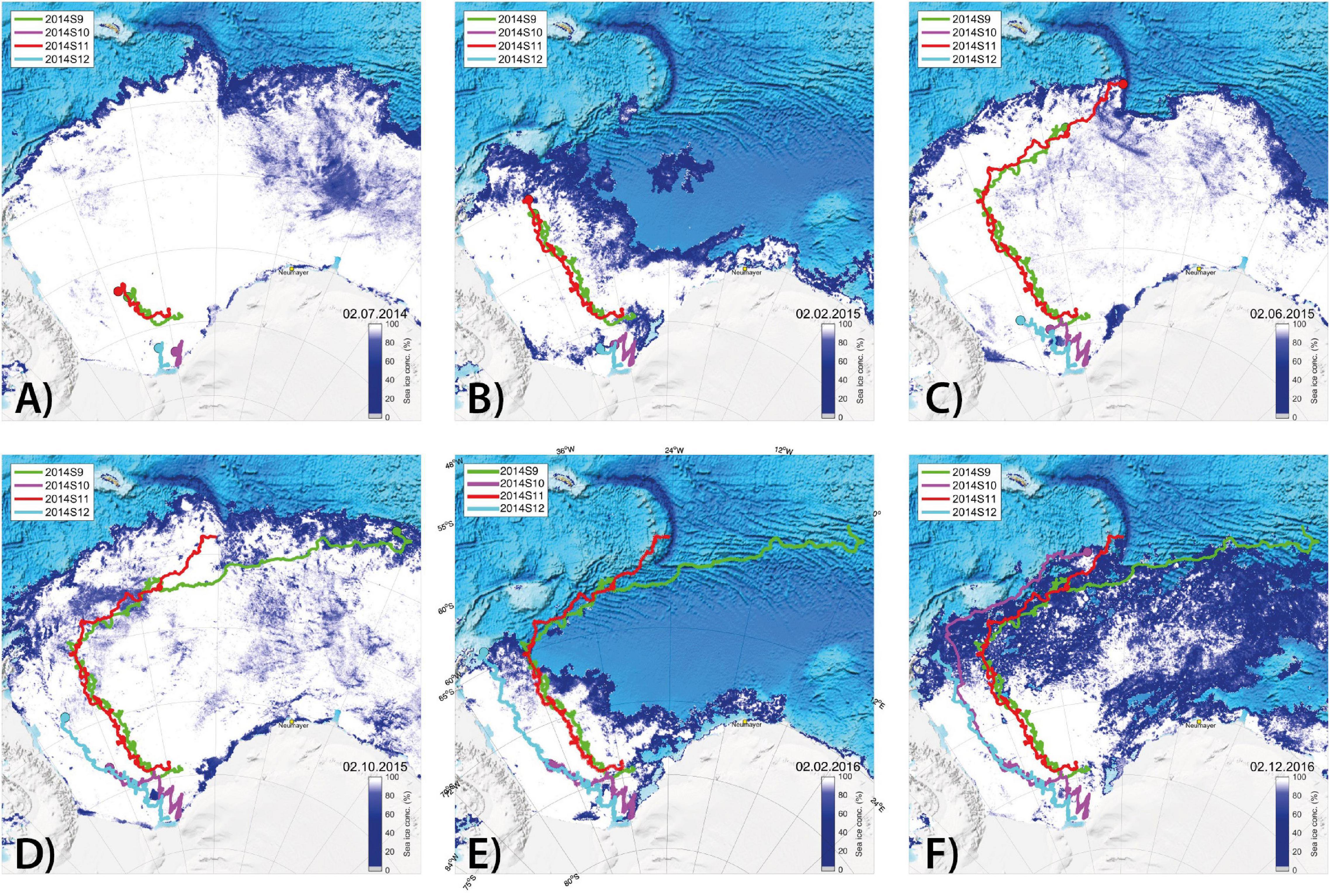
Figure 5. Maps of four Snow Buoys drifting through the Weddell Sea between January 2014 and December 2016. The plates show their positions at different times with the respective sea ice concentration in the background: (A) July 02, 2014 (after a few months), (B) February 02, 2015 (after 1 year), (C) June 02, 2015 (end of 2014S11), (D) October 02, 2015 (end of 2014S9), (E) February 02, 2016 (end of 2014S12), (F) December 02, 2016 (end of 2014S10). Active buoys (at the respective date) are indicated with an additional marker at the current position.
Buoys 2014S9 and 2014S11 were deployed approximately 250 km apart from each other and are herein referred to as the “northern pair.” Their separation was <250 km for more than 1 year before they separated toward the marginal ice zone. Buoys 2014S10 and 2014S12 (referred to as the “southern pair”) were deployed 500 km apart from each other and their separation was 500 to 800 km over the drift and thus much larger than of the northern pair. The barometric pressure and air temperature (data not shown) were almost identical for the northern pair and showed much larger differences for the buoys of the southern pair. Figure 6A shows the snow depth evolution recorded by all four buoys, indicating that snow accumulation was predominantly “event driven” with periods of several weeks with rather constant snow depth. Over the first year, both buoys of the northern pair measured a snow accumulation of approx. 0.45 m, while the initial snow depth was higher at buoy 2014S11. However, from September to December 2015 (austral spring), buoy 2014S11 measured an additional snow accumulation of 0.6 m while snow depth at buoy 2014S9 remained rather constant. Given the fact that both buoys should have experienced very similar atmospheric conditions, local topography effects are likely to have caused the additional accumulation at 2014S11. This accumulation led to almost coverage of 2014S11, causing the end of reliable data from this buoy. For 2014S9, snow depth reduced by about 0.20 m in summer before it increased by 0.30 m again. The net annual accumulation was 0.2 (0.9) m at 2014S9 (2014S11) between February 2014 and February 2015. In contrast, the southern pair shows comparable accumulation between the two buoys, although their separation was much greater than the northern pair. Over spring 2014, snow depth at 2014S10 and 2014S12 increased by 0.20–0.35 m. In the following summer, none of the buoys show a reduction in snow depth, instead snow depth at 2014S12 even increased by another 0.15 m. After 1 year (February 2014 to February 2015) both buoys accumulated approx. 0.75 m of snow. During the following year, 2014S10 and 2014S12 accumulated 0.6 and 0.0 m, respectively. However, the budget of 2014S12 might be split into two parts, an accumulation of 0.45 m until early December 2015 and a subsequent strong surface melt phase due to its location close to the ice edge and the onset of summer melt.
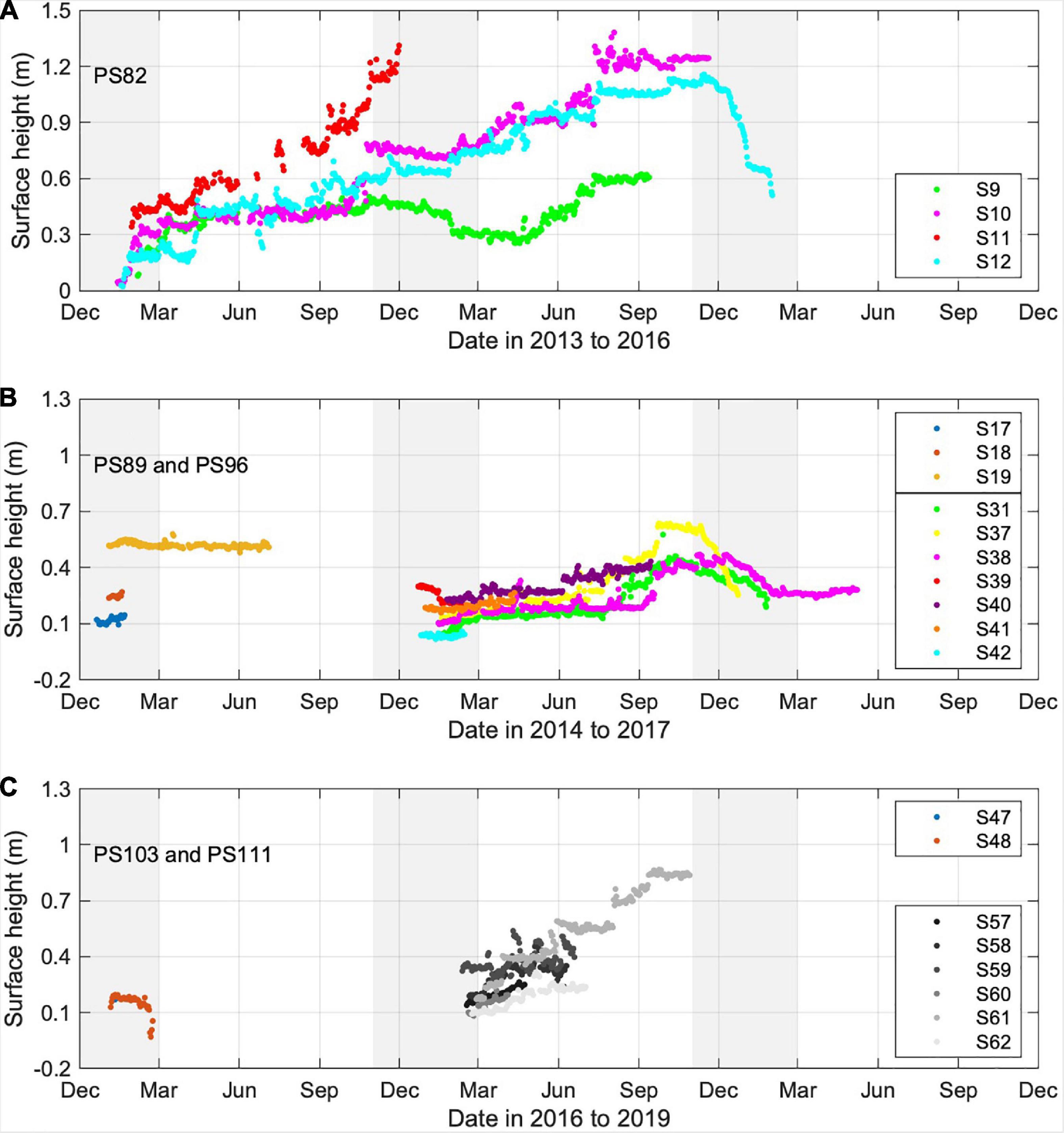
Figure 6. Daily mean surface height evolution from Snow Buoys on Antarctic sea ice. Different plates show groups of deployments during the expeditions (A) PS82, (B) PS89 and PS96, and (C) PS103 and PS111. The shaded areas indicate the potential melting period from December to March. Drift trajectories of individual buoys are shown in Figure 3 and in more detail in Supplementary Figures 4, 5 (using same colors). For shorter labels, buoy names do not include the year of deployment here, e.g., S31 is 2016S31.
Additional groups of Snow Buoys have been deployed in the Weddell Sea in the following years during the Polarstern expeditions PS89, PS96, PS103, and PS111. Their drift trajectories are shown in Figure 3 and in more detail in Supplementary Figure 6. Best results were obtained from the sets deployed during Polarstern expeditions PS96 in 2015/16 (Figure 6B) and PS111 in 2017/18 (Figure 6C). The PS96 set showed similar snow accumulation rates as observed in 2014, even though they were deployed slightly further north. Net accumulation of snow ranged from 0.35 to 0.60 m and was characterized by episodic snowfall events. However, some buoys stand out for particularly long times of almost no accumulation between February and September. Summer melt did not result in complete snow melt, while a strong surface ablation was only found for buoys close to the ice edge. The PS111 data set again exhibits the characteristic that one buoy (2018S61) shows much stronger accumulation than the rest of the set. It accumulated 0.7 m of snow between early March and end of October 2018 with the main accumulation of 0.5 m during the first 3 months. Again, we speculate that surface topography in the vicinity of the buoys played an important role in this. Unfortunately, the other buoys did not provide similarly long snow depth time series.
Air temperature for all these Weddell Sea buoys is shown in Figure 7. Lowest winter temperatures are around −30°C with few exceptions below. However, all four buoys that were active in the central Weddell Sea in August/September 2014 (see Figure 5A) showed temperatures well below −35°C for several weeks in this particular winter. Summer air temperatures vary between −5 and +5°C for all time series and are thus much less variable than winter temperatures. A strong warming is consistently observed for all buoys, starting early September until the maximum temperatures are reached in December. Autumn cooling sets in end of January/beginning of February in all cases, with weak dependence on the exact location or ice conditions.
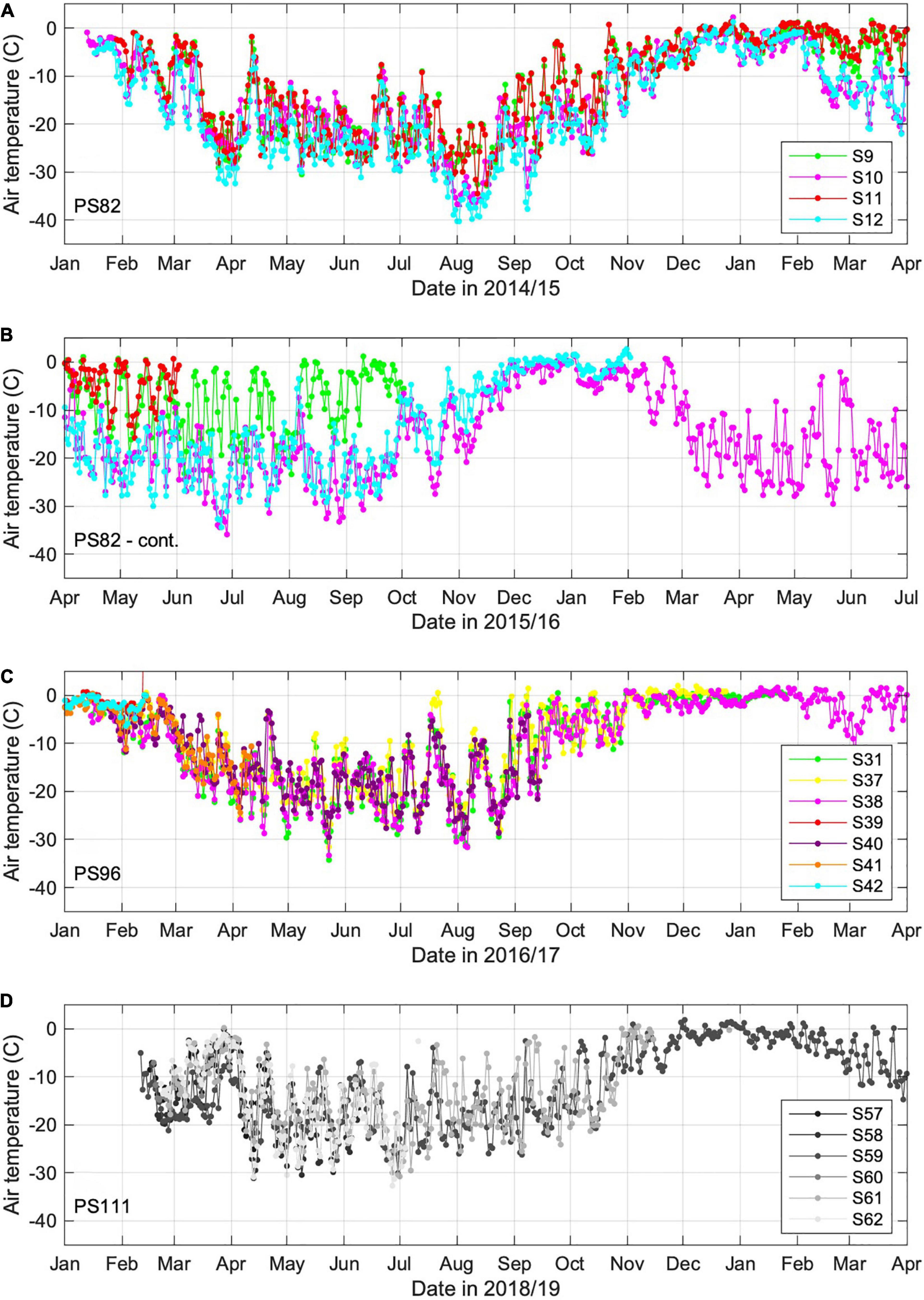
Figure 7. Daily mean air temperature over sea ice (height: approx. 1.5 m) recorded by Snow Buoys in the Antarctic Ocean. Different plates show groups of deployments during the expeditions (A) and (B) PS82, (C) PS96, and (D) PS111. Drift trajectories of individual buoys are shown in Figure 3 and in more detail in Supplementary Figures 4, 5 (using same colors). For shorter labels, buoy names do not include the year of deployment here, e.g., S36 is 2016S36. Note that the time series of PS82 is continued in plate (B).
Central Arctic Ocean Air Temperature and Snow Depth
Four sets of Snow Buoys were deployed in the central Arctic Ocean pack ice during summer/autumn 2015, 2016, and 2018. Figures 8, 9 show snow depth and air temperature from eight Snow Buoys that were installed during the Polarstern expedition PS94 in 2015, five during the Polarstern expedition PS101 in 2016, five from the Swedish ice breaker Oden during the expedition AO18 in 2018, and nine from the Russian ice breaker Akademik Tryoshnikov during the expedition T-ICE in 2018. Drift maps of all buoys are shown in Figure 3 and in more detail in Supplementary Figures 4, 5.
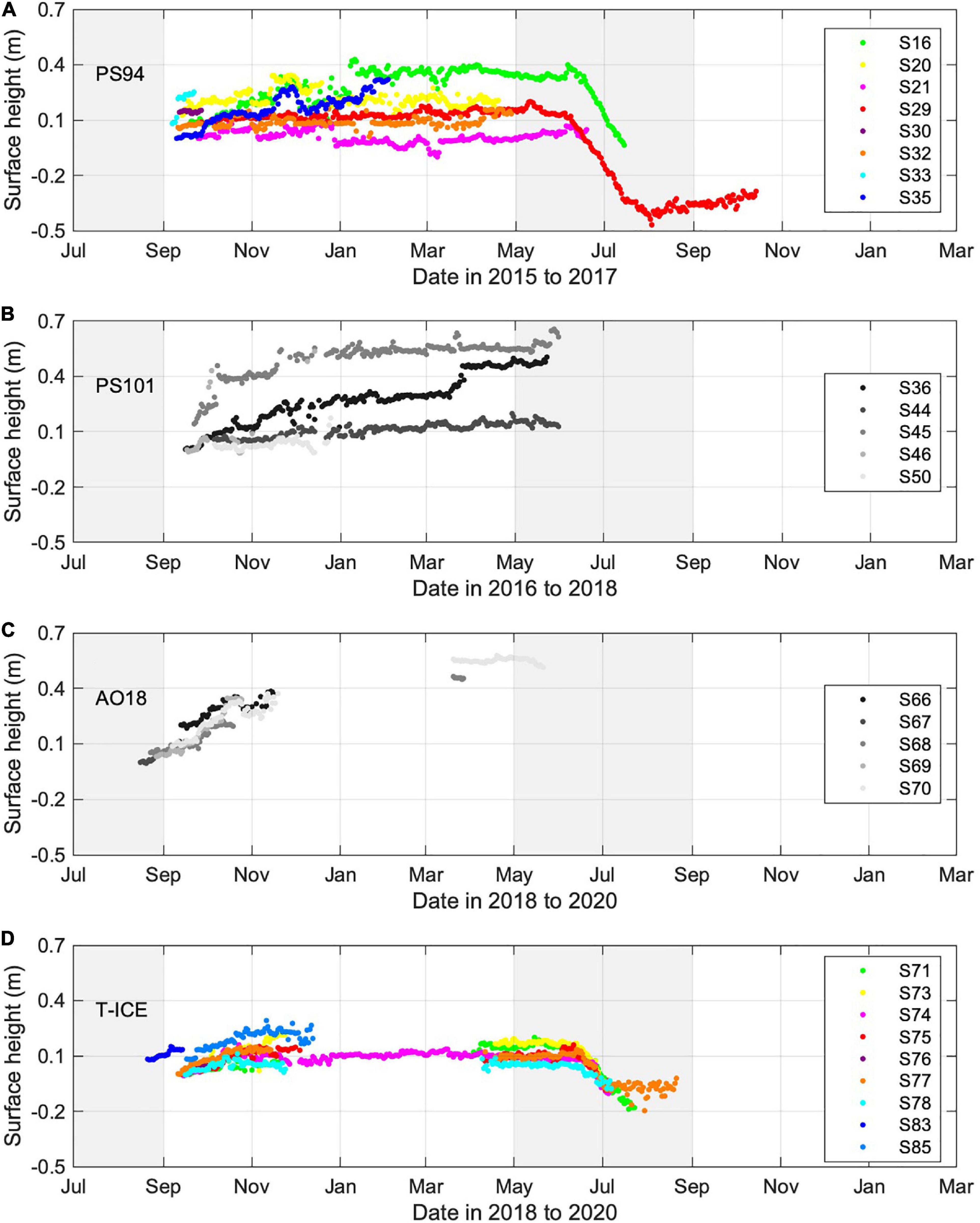
Figure 8. Daily mean surface height evolution from Snow Buoys on Arctic sea ice. Different plates show groups of deployments during the expeditions (A) P94, (B) PS101, (C) AO18, and (D) T-ICE. The shaded areas indicate the potential melting period from May to August in the Arctic. Drift trajectories of individual buoys are shown in Figure 3 and in more detail in the Supplementary Material. For shorter labels, buoy names do not include the year of deployment here, e.g., S16 is 2016S16.
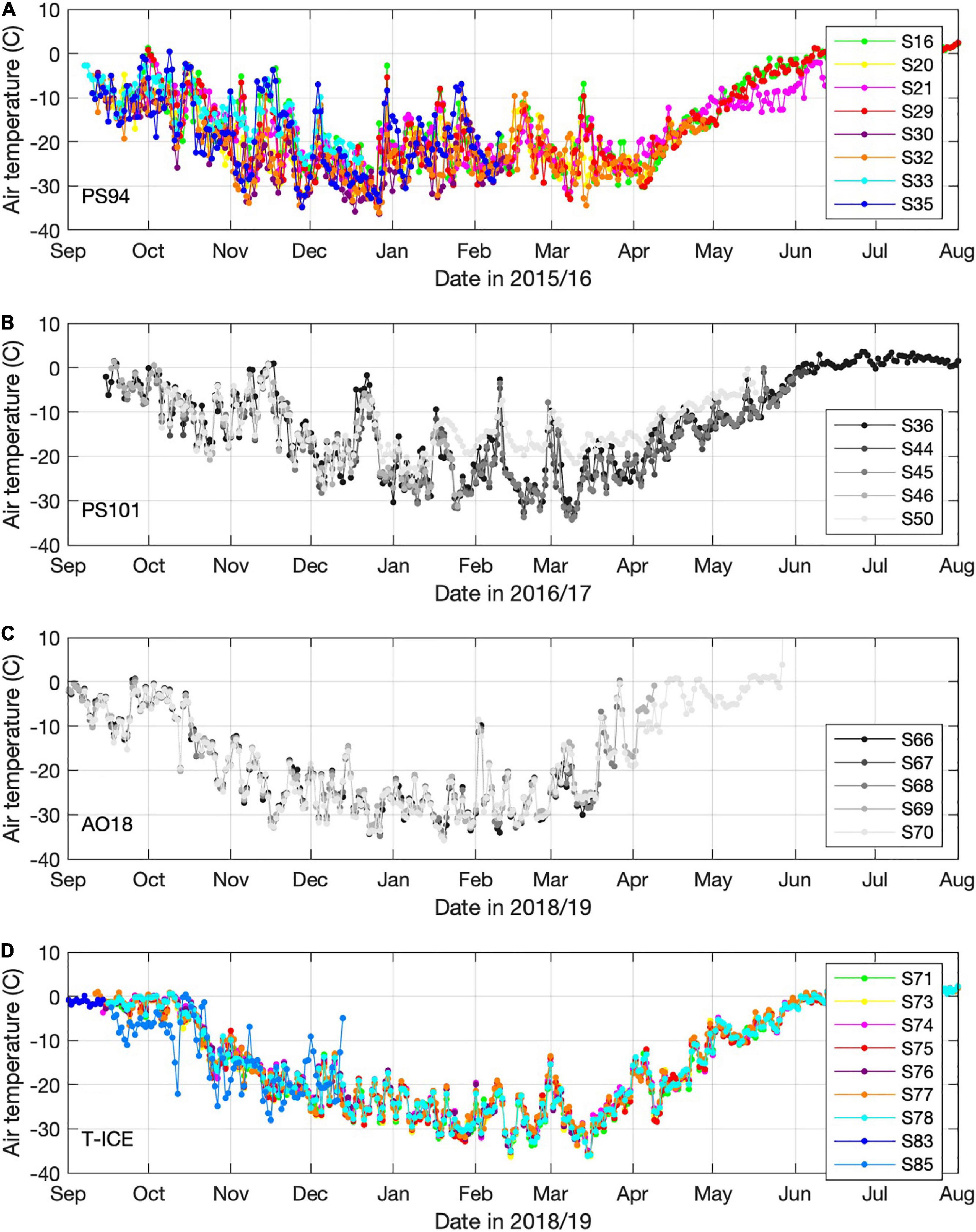
Figure 9. Daily mean air temperature (height: approx. 1.5 m) recorded by two sets of Snow Buoys in the Arctic Ocean. Different plates show groups of deployments during the expeditions (A) P94, (B) PS101, (C) AO18, and (D) T-ICE. Drift trajectories of individual buoys are shown in Figure 3 and in more detail in the Supplementary Material. For shorter labels, buoy names do not include the year of deployment here, e.g., S36 is 2016S36.
Here, we present and discuss the resulting snow depth time series with respect to the observed warm air events during winter (Boisvert et al., 2016; Gannon, 2016; Moore, 2016; Graham et al., 2017), which were captured by the Snow Buoys in 2016 and again in 2017. All of the corresponding time series are characterized by several pronounced temperature maxima, partially even exhibiting temperatures above freezing, close to the area around the North Pole during winter. The 2018/2019 buoys do not show such warm air events. Figure 9 shows the time series of daily mean temperatures, with strongest warming events observed in late December 2015 and early January 2016, as well as in November/December 2016 and February 2017. Individual measurements of hourly data sets exceed 0°C, mostly related to the passage of low pressure systems. However, these events were rather short and the high air temperatures did not translate into a decrease in snow depth as a result of surface melt (Figure 8). Instead, for 2015/2016, the snow depths from all six buoys in the area show a high variability throughout winter. Most buoys (2015S16, 2015S20, 2015S21, 2015S32, and 2015S35) show a net accumulation of max. 0.2 m over winter (Figure 8A), while 2015S20 and 2015S21 show some significant snow depth decrease in the range of 0.1 to 0.2 m in between. In addition, 2015S29 shows a similarly slow accumulation between October 2015 and April 2016, but then an increase in snow depth of 0.1 m within 2 weeks only (May), before a strong summer surface melt removes all snow and in addition the topmost 0.4 m of the sea ice. The accumulation pattern of 2015S16 was dominated by snowfall during winter and little change during spring, before summer melt in early June removed all snow again. 2015S30 and 2015S33 did not record valid snow data, most likely due to frosting on the sensors.
The buoys from 2016 started their drift further to the west and spread around Svalbard after deployment in a rather narrow region (Supplementary Figure 4). They showed higher snow accumulation over winter than the ones in the previous year, ranging from 0.1 to 0.5 m (Figure 8B). Similar accumulations were recorded from the 2018 buoys starting their drift from the North Pole region. Here it is remarkable that they captured a consistent snow accumulation of 0.4 m between August and end of November (Figure 8C). This is different to the set of buoys that drifted across the entire Transpolar Drift and spent autumn much further east. They only accumulated 0.2 m of snow in the same time window. The North Pole buoys continued to exhibit snow accumulation to up to 0.6 m by April, but only two buoys survived the winter season. The Transpolar Drift buoys had a higher survival rate through winter, with five buoys recording the melt of the entire snowpack and subsequent sea ice surface ablation. All 2018/2019 buoys, with one exception, have a data gap of snow readings of approx. 4 months during winter. This is most likely related to frost on the sensors, which seemed to be a predominant feature due to unfavorable atmospheric conditions. This lasted longer for the Transpolar Drift buoys, which were in higher latitudes for a longer period of time.
Discussion
Platform Performance
Integrating four ultrasonic range finders, increased accuracy and reliability compared to other platforms. Average operational time when using all four sensors was 204 days, while the average lifetime of a single range finder was only 187 days. Hence, the use of four ultrasonic range finders increased the amount of reliable data by approx. 10%. This is of particular interest given the high logistical efforts and costs associated to most deployments. Further advantages are their simple design, an easy deployment and immediate data availability. Snow Buoys are intentionally specialized and benefit from co-deployments of units that measure complementary parameters, e.g., ocean profilers, radiation stations, ice mass balance buoys, and position buoys of deformation arrays. Over the last two decades, time series of snow depth were mainly available from two other buoy types:
• In comparison to IMB (Richter-Menge et al., 2006), Snow Buoys are much cheaper, simpler in design and deployment, but Snow Buoys provide smaller parameter sets and do not provide sea ice thickness data. IMBs give also a more detailed profile of internal snow processes (e.g., snow metamorphism). Thus, Snow Buoys are often co-deployed with units that provide additional sea ice-thickness and snow measurements.
• In comparison to SIMBA-type thermistor string buoys (Jackson et al., 2013), Snow Buoys are of similar price and complexity. One of the main advantages of the ultrasonic range finder on the Snow Buoy is the direct detection of the air-snow interface, while it is quite challenging to derive this routinely from the thermistors. In addition, co-deployed units of both types will help to improve thermistor string buoy processing and interface detection (Cheng et al., 2020). Furthermore, air temperatures derived from thermistor string do only cover a few decimeters above the snow surface and radiative effects as well as frosting on the chain create stronger biases.
More comprehensive atmospheric data sets are e.g., available from Polar Atmospheric Weather Stations, which also carry wind direction and velocity as well as relative humidity measurements. Snow particle counters, as used by Leonard and Maksym (2011), would also add to more complex snow studies, but their addition was beyond the scope of the rather simple Snow Buoys so far.
In addition to the instrument itself, the Snow Buoy comes along with a data concept of standard processing, meta data of deployments (see Supplementary Table 1), and an open access data approach. All data are comprised in one place on www.meereisportal.de (Grosfeld et al., 2015), but also forwarding data into international networks [IABP, International Program for Antarctic Buoys (IPAB), and GTS]. Apart from improving global weather forecasts, this also provides a standard quality control, while the wide distribution allows many scientists to study recent weather events. Thus it is more likely to recognize special developments, such as the observed warm spells at the North Pole (Moore, 2016).
The ultrasonic range finders of the Snow Buoys give reliable measurements of the distance to the snow surface, at least under calm conditions (Figures 2, 4). Hence the uncertainty of the individual range measurement is in the range of millimeters. Larger scatter in these range measurements results from drifting/blowing snow, snow fall, and instrument icing resulting in apparently higher surfaces. These outliers may be filtered with rather basic methods and only few data sets show a particularly high noise level. The higher occurrence of noise in the Arctic (compared to the Antarctic) deployments during winter is likely related to enhanced frosting on the sensor and buoy structure due to higher air humidity. Largest uncertainties of snow depth measurements result from the conversion of range measurements to real snow depth, including the initial snow depth during deployment.
Air temperatures measured by the Snow Buoys exceed those measured at reference stations especially for low temperatures (summer: 1.4°C, winter: 2.9°C, Supplementary Figure 3). The main reason is likely the non-linear behavior of the thermistor element sensor. In order to overcome this effect, additional tests and pre-deployment calibration may be performed, but were not realized yet. Another typical source of errors, radiation effects during summer, were found to be of minor importance, although the Snow Buoy’s temperature sensor cannot be ventilated due to power limitations. These aspects have to be considered when using the un-corrected standard data product for air temperature measurements, as e.g., done in Moore (2016), when analyzing Arctic winter conditions based on GTS data. More work should be done to quantify this correction, also including general aspects on how to reduce biases on autonomous platforms compared to high quality manned reference stations.
Barometric pressure was found to be mostly lower than reference measurements with larger differences under high wind velocities. A classical explanation would be a strong influence based on Bernoulli’s Principle, describing that high winds cause a reduction in measured air pressure. However, since the pressure port is located in the body of the buoy, which is mostly buried in snow, the Bernoulli Principle should be strongly reduced. We are not able to give a general explanation for this difference, but mean pressure differences during times of low wind might be related to differences in the measurement height.
Seasonality and Regional Variability of Snow Depth on Sea Ice
Our experience shows that Snow Buoys can contribute to fill the critical gap of in situ snow depth and near-surface meteorological measurements in the remote ice-covered oceans. They will support a better understanding of snow and provide data that can be used for various model approaches and to develop better algorithms for satellite and airborne data products, as recently underlined e.g., by Webster et al. (2018) and Kwok et al. (2020). Other applications are improved estimates of surface radiation fluxes (Nicolaus et al., 2012; Arndt and Nicolaus, 2014) or the role of snow for sea ice growth (Merkouriadi et al., 2017) on different ice types. Snow accumulation and redistribution can be analyzed in more detail in connection with additional data sets from particle counters (Leonard and Maksym, 2011; Lecomte et al., 2015) or terrestrial laser scanning. Continuing the Snow Buoy program, changes on decadal time scales will be possible based on consistent time series from the different parts of the Arctic and Antarctic oceans (Webster et al., 2014).
In order to further discuss the results with respect to the spatial component, we separate the entire data set into four regional subsets, consisting of the more marginal and more central pack ice of the Arctic and Antarctic. We refer to them as “Arctic margin,” “Arctic center,” “Antarctic margin,” and “Antarctic center” for the purpose of this study. It should be noted that fewer time series were collected through the summer season in the Arctic compared to the Antarctic due to higher failure rates during the more intense melt seasons in the Arctic.
In the central Arctic, the accumulation period ranges from August to April, with a total accumulation of 30.5 cm (range: 10–50 cm) per year (Figure 10). Highest accumulation rates were found in September and October with 6.5 and 7.8 cm per month, respectively. Complete snow melt and a net loss of sea ice at the surface is a common feature on Arctic sea ice (Figure 8). Due to strong ablation in June and July of −14 and −8.7 cm, respectively, only a residual snow depth of 8.0 cm remains. In the marginal zones of the Arctic, the annual cycle is similar with highest accumulation rates in January and February. Summarizing, over the entire annual cycle only 3.4 cm are accumulated in lower Arctic latitudes. But it has to be noted that summer ablation is likely underestimated due buoys failing or falling over before the end of the ablation season. These findings are according to earlier findings from different studies. During the SHEBA drift campaign, the snow pack built up in October and November, attaining near-maximum depth (0.34 m) by mid-December with a rapid snow melt occurring from late May (Perovich et al., 1999). Snow Buoys from the N-ICE experiment were deployed on the existing snow cover of some 0.4 m depth during late winter and spring (Merkouriadi et al., 2017). Afterward they accumulated another 0.1–0.2 m before they also showed a strong surface melt. Also the Soviet stations and ice mass balance buoys, as e.g., described by Webster et al. (2014) and by re-analyses data an numerical studies as e.g., by Merkouriadi et al. (2017) or Stroeve et al. (2020). These differences are certainly strongly impacted by regional differences in the Arctic with different patterns in the Beaufort vs. Northern Atlantic regimes (Webster et al., 2018). A more detailed regional analysis is currently not possible due to lacking Snow Buoy data in the Beaufort region. But merging a larger set of snow depth from very different platforms and sources would e.g., allow to provide an additional update to the still frequently used snow climatology by Warren et al. (1999). Major improvements of the role of snow on Arctic sea ice and also on the spatial distribution of snow depth may be expected from the MOSAiC drift study, where also 20 Snow Buoys were part of the distributed network.
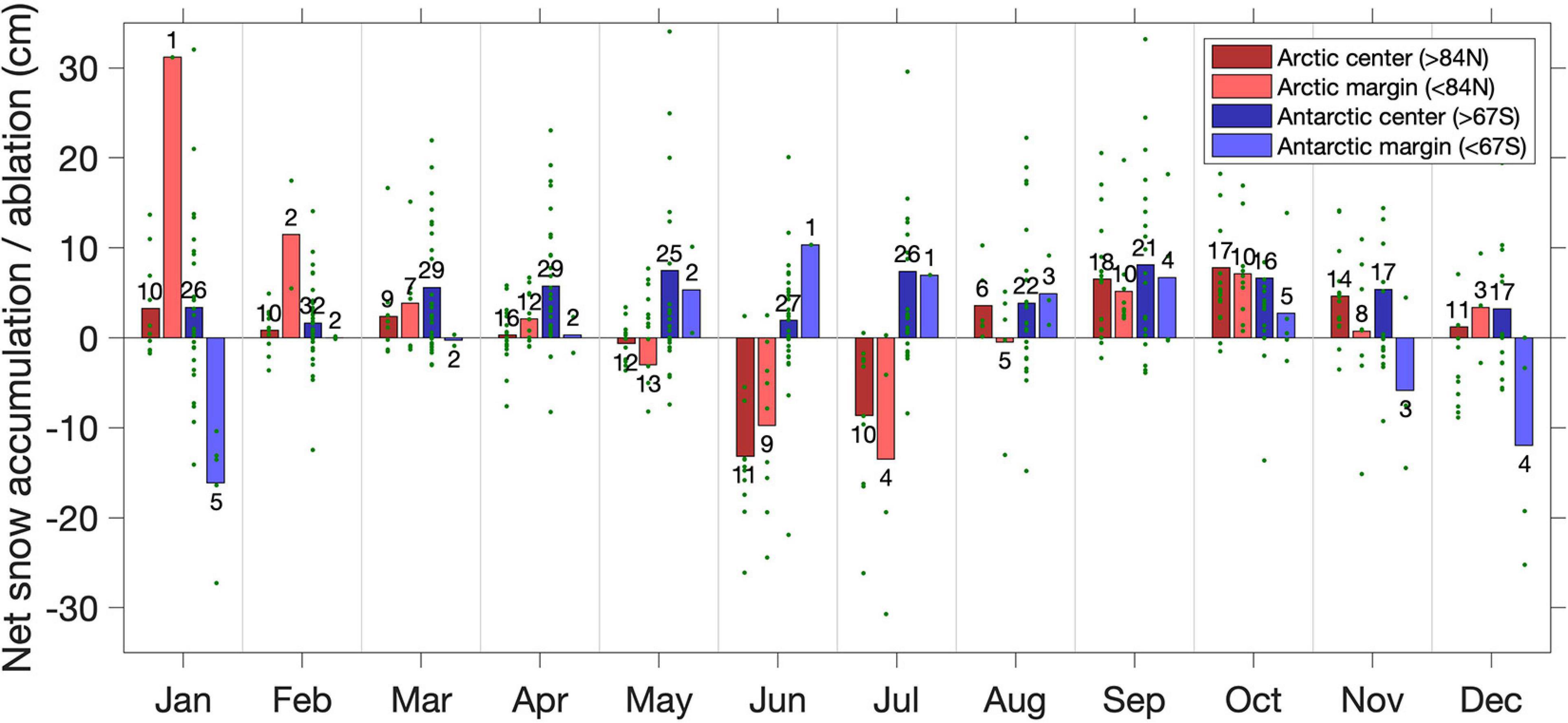
Figure 10. Mean monthly net accumulation (positive) or ablation (negative) of snow on sea ice in different regions of the Arctic and Antarctic. Net changes are distinguished between buoys in higher and lower latitudes. Small numbers indicate the number of buoys contributing to the mean value, while only buoys on drifting sea ice with minimum of 90 days of snow height data are included. Dots show each individual buoy. Note that mean values may include contributions from accumulation and ablation.
In the Antarctic, sea ice is well known for a year-around snow cover. We find that snow accumulation mainly occurs as episodic events and is highly variable from buoy to buoy. Accumulation events are irregularly distributed during the year and may include periods over more than 2 months with very little accumulation (Figure 6). Net accumulation rates ranged from 0.0 to 0.9 m. Several buoys reported an increase of snow depth even during summer, and none of the buoys reported ablation in the central Weddell Sea during summer. All buoys show a remaining net accumulation at the end of their life time, and complete melt or evaporation of the snow cover was not observed in the Antarctic. Only few buoys experienced a strong surface ablation, mostly due to snow melt in the marginal ice zone. Only Snow Buoys in the inner part of the Weddell Sea (Antarctic center) show snow accumulation in all months, including summer, with a total amount of 60.3 cm (Figure 10). The seasonal cycle is rather weak with accumulation rates between 2.0 and 8.1 cm per month, which is in agreement with the seasonal cycle of precipitation (Boisvert et al., 2020). This is in strong contrast to the lower latitudes in the Antarctic (Antarctic marginal), where summer ablation is observed (November to March) and the net annual accumulation is only 3.1 cm. Given the drift trajectories, a lot of snow accumulated in the inner parts of the Weddell Sea but are then lost in the outer parts again. Highest ablation takes place in December and January with a loss of 12.0 and 16.1 cm, respectively. This result refines the general finding of Massom et al. (2001) and updates it with measurements about two decades later. These results match well with the results by Arndt et al. (2016), who used satellite radiometry to show that strong internal melt is mostly observed in the marginal ice zone, while snow melt processes are much weaker in the inner part of the Weddell Sea. However, as discussed, our data are insufficient to distinguish between processes that contribute snow depth changes. Also, the snow observations during the Ice Station Polarstern (ISPOL, 2004/2005) show that the snow depth has increased until November, but compaction and melt reduced snow depth over summer until January. However, no entire loss of the snow pack was observed (Nicolaus et al., 2009). ISPOL took place in the western Weddell Sea, a region with expected surface melt, but without complete loss of the snow cover over summer (Willmes et al., 2011; Arndt et al., 2016).
Figure 11 shows the mean monthly air temperature in different regions of the Arctic and Antarctic. Both hemispheres show a pronounced seasonal cycle, as expected. Central Arctic air temperatures range from cold winter mean temperatures between −22.8 and −25.0°C from December to March to mean summer temperatures above freezing in July and August. June temperatures were positive in the marginal zones and only slightly negative for the central Arctic. The difference between lower and higher latitudes are less pronounced in the Arctic than in the Antarctic, where the monthly mean temperatures were >−15°C even during winter. Antarctic mean temperatures did not exceed 0°C during any month, although single buoys measured positive mean temperatures between November and February. Overall, the lowest mean temperatures were found for individual buoys in August in the Antarctic. Given the observed overestimation of low air temperatures, these temperatures need to be considered as an upper boundary for air temperatures over sea ice in winter.
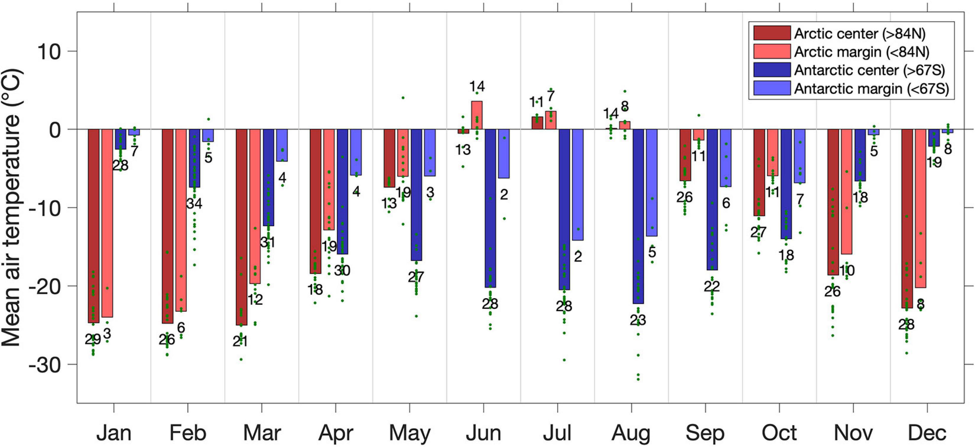
Figure 11. Mean monthly air temperature over sea ice in different regions of the Arctic and Antarctic. Only buoys on drifting sea ice with minimum of 90 days of air temperature data are included. Dots show each individual buoy.
Hidden Snow Processes Impacting Snow Depth
The comparison of the two buoy pairs that drifted through the Weddell Sea highlights that local effects, such as surface topography, may have a high impact on snow depth. This is not surprising, but it is obviously a feature that requires more investigation. This raises the question on how much time series data from level ice can represent the overall snow mass distribution. There are indications that the role of snow associated to ridges and deformation areas have a much higher contribution than considered in most studies so far. Sturm et al. (2002) found that snow depth at SHEBA was 30% higher in ridges than on level ice. In addition, the surface fraction of ridges would be needed to estimate the total snow volume caught in ridges.
Another feature that becomes obvious from the Antarctic buoys is the role of snow-ice and superimposed ice formation, as well as flooding or gap layer formation. They do not necessarily change the surface elevation, but the thickness of the pure snow layer, and thus what is mostly considered as “snow depth.” In this study, we found particularly high accumulation rates, and thus also very high total snow depth, on sea ice in the Weddell Sea (Figure 6). An increase of surface elevation of up to 1.4 m was observed by 2014S10 (Figure 2) over the 2.5 years of drift. But in order to sustain a dry snow ice interface based on the isostatic equilibrium, sea ice thickness had to increase from 1.32 m (0.12 m freeboard, Table 2) to more than 3.90 m (assuming a freeboard of 0.00 m) in the same timeframe. For the given conditions, this is very unlikely and shows that data interpretation of these snow depth measurements needs to account for changes and conversion processes at the snow/ice interface. This conversion of surface height measurements to snow depth is a well-known issue also for laser altimetry during airborne missions or from surface scanning. In this study, we consider the snow/ice interface to be stable and any positive change in surface height is regarded as snow. This assumption is made due to the lack of additional information. For the future, such information may be retrieved either from co-deployed high-resolution thermistor string buoys (Provost et al., 2017; Cheng et al., 2020).
In addition to observational data, complementary information on snow/ice interface processes over time may be derived from the application of a thermodynamical snow and sea ice model. The presented time series may add to such studies and thus create a better process understanding, e.g., by coupling trajectory data from Snow Buoys with numerical models as done by Nicolaus et al. (2006) or by Wever et al. (2020).
Most of the findings discussed here are based on the results and discussion of the mean snow depth. However, further analysis will also look into the variability between the four sensors, as shown in Figure 2. They will provide insights into the variability of snow depth and accumulation on meter scale, as well as on data quality. At the same time, data sets will be able to define the variability within the four measurements and how this variability might change seasonally. Co-deployments of several Snow Buoys on one floe and/or the combination with snow depth data from other buoy types may also allow distinguishing accumulation through snowfall and snowdrift.
Winter Warm Spells and Their Effects on Arctic Snow Packs
The two sets of Snow Buoys deployed in the central Arctic in 2015 and 2016 (Figures 8, 9) contributed to a comparably good spatial and temporal coverage of meteorological and snow depth measurements over this otherwise sparsely sampled region. The time series of air temperature measurements of those buoys revealed the passage of several warm synoptic systems over the central Arctic (Graham et al., 2017). Since there are no permanent weather stations anywhere in the central Arctic Ocean, the buoys’ hourly provision of air temperature and barometric pressure measurements to the GTS and the IABP database were crucial in better estimating the conditions during one of the most anomalous winters in recent history in this region. The temperature evolution in late December for example was the consequence of a powerful winter cyclone (or “freak storm,” as entitled by the Washington Post on December 30, 2015), which brought temperatures above freezing even close to the North Pole (Gannon, 2016; Moore, 2016). A similar event was recorded in February 2017, again exceeding the melting point in the region north of Svalbard (Graham et al., 2017). At least in the central Arctic, these high air temperatures did not lead to a consistent decrease in snow depth. Despite the overall absence of pronounced surface melt, the warm winter conditions led to an overall decreased sea ice growth rate. Linking Snow Buoy snow depth and air temperature data into numerical models of the snow pack, it will be possible to investigate the role of these warm spells for the snow pack in more detail. This process was also described by Merkouriadi et al. (2020) based on the N-ICE data in 2015. Snow packs that experienced such warm spells might experience increased metamorphism and compaction, which then impact the properties of the snow pack later in the seasons. This will likely impact (reduce) the chance for redistribution of the otherwise more loose snow and alter optical properties with respect to surface energy budgets.
Conclusion and Outlook
The Snow Buoy is a new tool to obtain autonomous measurements of snow depth, air temperature and barometric pressure in sea ice environments. Key components are four ultrasonic range finders measuring surface height that is converted into snow depth. Between 2013 and 2019, 79 buoys were deployed in the Arctic Ocean and Weddell Sea, some of which provided the longest autonomous time series of snow depth on Weddell Sea pack ice and probably the most comprehensive in situ data set of snow depth on Antarctic sea ice so far. Main uncertainties result from the tilt of stations and that hidden snow metamorphism and snow-ice transition cannot be monitored.
A standard data processing has been established which generates open access, high quality, and consistent datasets, allowing us to draw conclusions on hemispherical and regional differences in snow depth seasonality as long as “hidden” processes of snow metamorphism and freeboard changes are considered. Availability of the data in near-real time allows alerting the general public of the Arctic warming event in December 2015 and January 2017.
In the Weddell Sea, annual snow net accumulation ranged from 0.2 to 0.9 m. The annual cycle is characterized by episodic accumulation and only weak summer melt, except for the marginal ice zone. The inner part of the Weddell Sea shows only a weak seasonal cycle with snow accumulation in all months, including summer. On Arctic sea ice, annual net accumulation was only 0.1 to 0.4 m with complete snow melt and partial surface ablation of the sea ice.
The program is planned to be continued and established over the coming years based on collaborations within the IABP and the IPAB. A major extension of the time series is realized during the MOSAiC drift from October 2019 to September 2020 with an additional 20 installations.
Future studies are suggested for merging spatial data sets with these time series in order to quantify how representative point measurements on level ice are in comparison to the snow cover on the complex and ridged pack ice. Studies benefiting from this dataset include an investigation of small-scale processes, large-scale (basin wide) snow seasonality on sea ice as well as the validation of satellite data and numerical model studies. In addition, more knowledge on the “hidden” processes at the snow/ice interface and the relation of snow depth and surface height is needed. Here we suggest the combination with one-dimensional snow pack/sea ice models, forced with re-analysis data along the trajectories, and co-deployments with IMBs of different kinds.
Data Availability Statement
The datasets presented in this study can be found under https://doi.org/10.1594/PANGAEA.875272.
Author Contributions
MN and MH initiated this manuscript and prepared all figures. MN, MS, MH, CK, and SH were involved in developing the prototype buoy and developed the data processing. AN compiled the data set and coordinated the data flow and publication. All authors contributed to analyzing different parts of the data set, discussing the methods and results, and were directly contributing to writing the manuscript.
Funding
All buoys highlighted in this article were funded by the Helmholtz infrastructure programs ACROSS and FRAM. Different authors received funding from external projects: Helmholtz Alliance “Remote Sensing and Earth System Dynamics” (HA-310), EU H2020 project SPICES (640161), EU FP7-SPACE project SIDARUS (262922), DFG projects SIMBIS (NI1096/2-1), SCASI (NI1096/5-1), and SnowCast (AR1236/1), ESA Sea Ice CCI phase 1 and 2 (AO/1-6772/11/I-AM), and the German Ministry of Economics and Technology (50EE1008). We highly appreciate the work of the www.meereisportal.de team for building and maintaining the online platform and database for all Snow Buoy data and figures (REKLIM-2012-04).
Conflict of Interest
The authors declare that the research was conducted in the absence of any commercial or financial relationships that could be construed as a potential conflict of interest.
Acknowledgments
We strongly acknowledge the support of the captains, the crews, the helicopter teams, and the scientific cruise leaders Michael Schröder (PS82, Grant No: AWI_PS82_02 and PS96, Grant No: AWI_PS96_01), Olaf Boebel (PS89, Grant No: AWI-PS89_02), Ursula Schauer (PS94, Grant No: AWI_PS94_00), and Antje Boetius (PS101, Grant No: AWI_PS100_01) of RV Polarstern expeditions for their help and support. In the same way, we acknowledge the work of the captains, the crews and the scientific parties of the expeditions AO18 with the Swedish Icebreaker Oden and T-ICE with the Russian ice breaker Akademik Tryoshnikov (Grant No: 63A0028B). The wintering teams at Neumayer III base helped greatly to improve the Snow Buoy and to obtain the long time series close to the station (mainly buoy 2013S2). We are grateful to Thomas Lavergne, as a main user of the online data sets, to help us improving the data sets and Hauke Schulz for his comments on the manuscript with respect to the BSRN measurements. Georg Heygster and Marcus Huntemann (University of Bremen) as well as Nina Maaß (University of Hamburg) gave valuable contributions by discussing the buoy measurements with respect to comparisons with remote sensing data products. The deployments of various Snow Buoys benefited from the logistics and support of many partners and Institutes: Norwegian Polar Institute (in particular the N-ICE 2015 experiment), University of Alaska, Swedish Polar Research Secretariat, Universität Hamburg, CH2MHill Polar Services, Barrow Arctic Science Consortium, and UMIAQ. Danielle Langevin and her team of MetOcean Telematics (Halifax, Canada) contributed significantly to the development and stepwise improvement of the Snow Buoys, as well as the timely shipment to the various deployments. Sea ice concentration, as used in the maps as background data, is kindly provided by the Universität Bremen (Institut für Umweltphysik). The prototypes and development of the Snow Buoy were financed by the Alfred-Wegener-Institut.
Supplementary Material
The Supplementary Material for this article can be found online at: https://www.frontiersin.org/articles/10.3389/fmars.2021.655446/full#supplementary-material
Footnotes
References
Abraham, C., Steiner, N., Monahan, A., and Michel, C. (2015). Effects of subgrid-scale snow thickness variability on radiative transfer in sea ice. J. Geophys. Res. Oceans 120, 5597–5614. doi: 10.1002/2015jc010741
Armitage, T. W. K., and Ridout, A. L. (2015). Arctic sea ice freeboard from AltiKa and comparison with CryoSat-2 and Operation IceBridge. Geophys. Res. Lett. 42, 6724–6731. doi: 10.1002/2015gl064823
Arndt, S., and Nicolaus, M. (2014). Seasonal cycle of solar energy fluxes through Arctic sea ice. Cryosphere Dis. 8, 2923–2956.
Arndt, S., and Paul, S. (2018). Variability of Winter Snow Properties on Different Spatial Scales in the Weddell Sea. J. Geophys. Res. Oceans 123, 8862–8876. doi: 10.1029/2018jc014447
Arndt, S., Meiners, K. M., Ricker, R., Krumpen, T., Katlein, C., and Nicolaus, M. (2017). Influence of snow depth and surface flooding on light transmission through Antarctic pack ice. J. Geophys. Res. Oceans 122, 2108–2119. doi: 10.1002/2016jc012325
Arndt, S., Willmes, S., Dierking, W., and Nicolaus, M. (2016). Timing and regional patterns of snowmelt on Antarctic sea ice from passive microwave satellite observations. J. Geophys. Res. Oceans 121, 5916–5930. doi: 10.1002/2015jc011504
Behrendt, A., Dierking, W., and Witte, H. (2015). Thermodynamic sea ice growth in the central Weddell Sea, observed in upward-looking sonar data. J. Geophys. Res. Oceans 120, 2270–2286. doi: 10.1002/2014jc010408
Boisvert, L. N., Petty, A. A., and Stroeve, J. C. (2016). The Impact of the Extreme Winter 2015/16 Arctic Cyclone on the Barents–Kara Seas. Monthly Weather Rev. 144, 4279–4287. doi: 10.1175/mwr-d-16-0234.1
Boisvert, L. N., Webster, M. A., Petty, A. A., Markus, T., Cullather, R. I., and Bromwich, D. H. (2020). Intercomparison of Precipitation Estimates over the Southern Ocean from Atmospheric Reanalyses. J. Clim. 33, 10627–10651. doi: 10.1175/jcli-d-20-0044.1
Castro-Morales, K., Kauker, F., Losch, M., Hendricks, S., Riemann-Campe, K., and Gerdes, R. (2014). Sensitivity of simulated Arctic sea ice to realistic ice thickness distributions and snow parameterizations. J. Geophys. Res. Oceans 119, 559–571. doi: 10.1002/2013jc009342
Cheng, Y., Cheng, B., Zheng, F., Vihma, T., Kontu, A., Yang, Q., et al. (2020). Air/snow, snow/ice and ice/water interfaces detection from high-resolution vertical temperature profiles measured by ice mass-balance buoys on an Arctic lake. Ann. Glaciol. 2020, 1–11. doi: 10.1017/aog.2020.51
Gearheard, S., Matumeak, W., Angutikjuaq, I., Maslanik, J., Huntington, H. P., Leavitt, J., et al. (2006). “It’s not that simple”: A collaborative comparison of sea ice environments, their uses, observed changes, and adaptations in barrow, Alaska, USA, and Clyde River, Nunavut, Canada. Ambio 35, 203–211. doi: 10.1579/0044-7447(2006)35[203:intsac]2.0.co;2
Gerland, S., and Haas, C. (2011). Snow-depth observations by adventurers traveling on Arctic sea ice. Ann. Glaciol. 52, 369–376. doi: 10.3189/172756411795931552
Graham, R. M., Cohen, L., Petty, A. A., Boisvert, L. N., Rinke, A., Hudson, S. R., et al. (2017). Increasing frequency and duration of Arctic winter warming events. Geophys. Res. Lett. 44, 6974–6983. doi: 10.1002/2017gl073395
Granskog, M. A., Assmy, P., Gerland, S., Spreen, G., Steen, H., and Smedsrud, H. L. (2016). Arctic research on thin ice: Consequences of Arctic sea ice loss. EOS 97, 22–26.
Granskog, M. A., Rösel, A., Dodd, P. A., Divine, D. V., Gerland, S., Martma, T., et al. (2017). Snow contribution to first-year and second-year Arctic sea ice mass balance north of Svalbard. J. Geophys. Res. Oceans 2017:12398. doi: 10.1002/2016JC012398
Grenfell, T. C., Light, B., and Sturm, M. (2002). Spatial distribution and radiative effects of soot in the snow and sea ice during the SHEBA experiment. J. Geophys. Res. Oceans 107:414.
Grosfeld, K., Treffeisen, R., Asseng, J., Bartsch, A., Bräuer, B., Fritzsch, B., et al. (2015). Online sea-ice knowledge and data platform. Polarforschung 85, 143–155.
Guerreiro, K., Fleury, S., Zakharova, E., Remy, F., and Kouraev, A. (2016). Potential for estimation of snow depth on Arctic sea ice from CryoSat-2 and SARAL/AltiKa missions. Remote Sens. Environ. 186, 339–349. doi: 10.1016/j.rse.2016.07.013
Haas, C., Nicolaus, M., Willmes, S., Worby, A., and Flinspach, D. (2008). Sea ice and snow thickness and physical properties of an ice floe in the western Weddell Sea and their changes during spring warming. Deep Sea Res. II 55, 963–974. doi: 10.1016/j.dsr2.2007.12.020
Haas, C., Thomas, D. N., and Bareiss, J. (2001). Surface properties and processes of perennial Antarctic sea ice in summer. J. Glaciol. 47, 613–625. doi: 10.3189/172756501781831864
Heil, P. (2006). Atmospheric conditions and fast ice at Davis, East Antarctica: A case study. J. Geophys. Res. Oceans 111:2904.
Hellmer, H. H., Schröder, M., Haas, C., Dieckmann, G. S., and Spindler, M. (2008). The ISPOL drift experiment. Deep Sea Res. II 55, 913–917. doi: 10.1016/j.dsr2.2008.01.001
Hoppmann, M., Nicolaus, M., Hunkeler, P. A., Heil, P., Behrens, L. K., Konig-Langlo, G., et al. (2015). Seasonal evolution of an ice-shelf influenced fast-ice regime, derived from an autonomous thermistor chain. J. Geophys. Res. Oceans 120, 1703–1724. doi: 10.1002/2014jc010327
Itkin, P., Spreen, G., Cheng, B., Doble, M., Girard-Ardhuin, F., Haapala, J., et al. (2017). Thin ice and storms: Sea ice deformation from buoy arrays deployed during N-ICE2015. J. Geophys. Res. Oceans 2017:12403. doi: 10.1002/2016JC012403
Jackson, K., Wilkinson, J., Maksym, T., Meldrum, D., Beckers, J., Haas, C., et al. (2013). A Novel and Low-Cost Sea Ice Mass Balance Buoy. J. Atmos. Ocean Tech. 30, 2676–2688. doi: 10.1175/jtech-d-13-00058.1
Jacobi, H. W., Voisin, D., Jaffrezo, J. L., Cozic, J., and Douglas, T. A. (2012). Chemical composition of the snowpack during the OASIS spring campaign 2009 at Barrow, Alaska. J. Geophys. Res. Atmospher. 117:6654.
Kern, M., Cullen, R., Berruti, B., Bouffard, J., Casal, T., Drinkwater, M. R., et al. (2020). The Copernicus Polar Ice and Snow Topography Altimeter (CRISTAL) high-priority candidate mission. Cryosphere 14, 2235–2251. doi: 10.5194/tc-14-2235-2020
Kern, S., and Ozsoy-Cicek, B. (2016). Satellite Remote Sensing of Snow Depth on Antarctic Sea Ice: An Inter-Comparison of Two Empirical Approaches. Remote Sens Basel 8:450. doi: 10.3390/rs8060450
King, J., Skourup, H., Hvidegaard, S. M., Rösel, A., Gerland, S., Spreen, G., et al. (2018). Comparison of Freeboard Retrieval and Ice Thickness Calculation From ALS, ASIRAS, and CryoSat-2 in the Norwegian Arctic to Field Measurements Made During the N-ICE2015 Expedition. J. Geophys. Res. Oceans 123, 1123–1141. doi: 10.1002/2017jc013233
König-Langlo, G. (2017). Meteorological synoptical observations from Neumayer Station, 2013-01 to 2016-01. Bremerhaven: Alfred Wegener Institute.
König-Langlo, G., and Raffel, B. (2017). High resolved snow height measurements at Neumayer Station, Antarctica, 2013 - 2015. Bremerhaven: Alfred Wegener Institute.
Krumpen, T., Birrien, F., Kauker, F., Rackow, T., von Albedyll, L., Angelopoulos, M., et al. (2020). The MOSAiC ice floe: sediment-laden survivor from the Siberian shelf. Cryosphere 14, 2173–2187. doi: 10.5194/tc-14-2173-2020
Kurtz, N. T., and Farrell, S. L. (2011). Large-scale surveys of snow depth on Arctic sea ice from Operation IceBridge. Geophys. Res. Lett. 38:49216.
Kurtz, N. T., Galin, N., and Studinger, M. (2014). An improved CryoSat-2 sea ice freeboard retrieval algorithm through the use of waveform fitting. Cryosphere 8, 1217–1237. doi: 10.5194/tc-8-1217-2014
Kwok, R. (2014). Simulated effects of a snow layer on retrieval of CryoSat-2 sea ice freeboard. Geophys. Res. Lett. 41, 5014–5020. doi: 10.1002/2014gl060993
Kwok, R., and Cunningham, G. F. (2008). ICESat over Arctic sea ice: Estimation of snow depth and ice thickness. J. Geophys. Res. Oceans 113:C08010.
Kwok, R., Kacimi, S., Webster, M. A., Kurtz, N. T., and Petty, A. A. (2020). Arctic Snow Depth and Sea Ice Thickness From ICESat-2 and CryoSat-2 Freeboards: A First Examination. J. Geophys. Res. Oceans 125:e2019JC016008.
Kwok, R., Zwally, H. J., and Yi, D. (2004). ICESat observations of Arctic sea ice: A first look. Geophys. Res. Lett. 31:20309.
Lawrence, I. R., Tsamados, M. C., Stroeve, J. C., Armitage, T. W. K., and Ridout, A. L. (2018). Estimating snow depth over Arctic sea ice from calibrated dual-frequency radar freeboards. Cryosphere 12, 3551–3564. doi: 10.5194/tc-12-3551-2018
Lecomte, O., Fichefet, T., Flocco, D., Schroeder, D., and Vancoppenolle, M. (2015). Interactions between wind-blown snow redistribution and melt ponds in a coupled ocean-sea ice model. Ocean Model. 87, 67–80. doi: 10.1016/j.ocemod.2014.12.003
Lecomte, O., Fichefet, T., Vancoppenolle, M., and Nicolaus, M. (2011). A new snow thermodynamic scheme for large-scale sea-ice models. Ann. Glaciol. 52, 337–346. doi: 10.3189/172756411795931453
Lei, R. B., Li, Z. J., Cheng, B., Zhang, Z. H., and Heil, P. (2010). Annual cycle of landfast sea ice in Prydz Bay, east Antarctica. J. Geophys. Res. Oceans 115:5223.
Leonard, K. C., and Maksym, T. (2011). The importance of wind-blown snow redistribution to snow accumulation on Bellingshausen Sea ice. Ann. Glaciol. 52, 271–278. doi: 10.3189/172756411795931651
Liston, G. E., Polashenski, C., Rösel, A., Itkin, P., King, J., Merkouriadi, I., et al. (2018). A Distributed Snow-Evolution Model for Sea-Ice Applications (SnowModel). J. Geophys. Res. Oceans 123, 3786–3810. doi: 10.1002/2017jc013706
Massom, R. A., Eicken, H., Haas, C., Jeffries, M. O., Drinkwater, M. R., Sturm, M., et al. (2001). Snow on Antarctic sea ice. Rev. Geophys. 39, 413–445.
Merkouriadi, I., Cheng, B., Graham, R. M., Rosel, A., and Granskog, M. A. (2017). Critical Role of Snow on Sea Ice Growth in the Atlantic Sector of the Arctic Ocean. Geophys. Res. Lett. 44, 10479–10485.
Merkouriadi, I., Cheng, B., Hudson, S. R., and Granskog, M. A. (2020). Effect of frequent winter warming events (storms) and snow on sea-ice growth – a case from the Atlantic sector of the Arctic Ocean during the N-ICE2015 campaign. Ann. Glaciol. 61, 164–170. doi: 10.1017/aog.2020.25
Moore, G. W. K. (2016). The December 2015 North Pole Warming Event and the Increasing Occurrence of Such Events. Sci. Rep. 6:39084.
Nandan, V., Geldsetzer, T., Yackel, J., Mahmud, M., Scharien, R., Howell, S., et al. (2017). Effect of Snow Salinity on CryoSat-2 Arctic First-Year Sea Ice Freeboard Measurements. Geophys. Res. Lett. 44, 10419–10426.
Nicolaus, M., Gerland, S., Hudson, S. R., Hanson, S., Haapala, J., and Perovich, D. K. (2010). Seasonality of spectral albedo and transmittance as observed in the Arctic Transpolar Drift in 2007. J. Geophys. Res. Oceans 115:6074.
Nicolaus, M., Haas, C., and Willmes, S. (2009). Evolution of first-year and second-year snow properties on sea ice in the Weddell Sea during spring-summer transition. J. Geophys. Res. 114:11227.
Nicolaus, M., Haas, C., Bareiss, J., and Willmes, S. (2006). A model study of differences of snow thinning on Arctic and Antarctic first-year sea ice during spring and summer. Ann. Glaciol. 44, 147–153. doi: 10.3189/172756406781811312
Nicolaus, M., Hoppmann, M., Arndt, S., Hendricks, S., Katlein, C., König-Langlo, G., et al. (2017). Snow height and air temperature on sea ice from Snow Buoy measurements. Bremerhaven: Alfred Wegener Institute.
Nicolaus, M., Katlein, C., Maslanik, J., and Hendricks, S. (2012). Changes in Arctic sea ice result in increasing light transmittance and absorption. Geophys. Res. Lett. 39:L24501.
Ozsoy-Cicek, B., Kern, S., Ackley, S. F., Xie, H. J., and Tekeli, A. E. (2011). Intercomparisons of Antarctic sea ice types from visual ship, RADARSAT-1 SAR, Envisat ASAR, QuikSCAT, and AMSR-E satellite observations in the Bellingshausen Sea. Deep Sea Res. Part II Topic. Stud. Oceanogr. 58, 1092–1111. doi: 10.1016/j.dsr2.2010.10.031
Perovich, D. K., Andreas, W. L., Curry, J. A., Eicken, H., Fairall, C. W., Grenfell, T. C., et al. (1999). Year on ice gives climate insights. Eos Transact. 80, 485–486.
Provost, C., Sennéchael, N., Miguet, J., Itkin, P., Rösel, A., Koenig, Z., et al. (2017). Observations of flooding and snow-ice formation in a thinner Arctic sea ice regime during the N-ICE2015 campaign: Influence of basal ice melt and storms. J. Geophys. Res. Oceans 2017:12011. doi: 10.1002/2016JC012011
Richter-Menge, J., Perovich, D. K., Elder, B. C., Claffey, K., Rigor, I., and Ortmeyer, M. (2006). Ice mass-balance buoys: a tool for measuring and attributing changes in the thickness of the Arctic sea-ice cover. Ann. Glaciol. 44, 205–210. doi: 10.3189/172756406781811727
Ricker, R., Hendricks, S., Perovich, D. K., Helm, V., and Gerdes, R. (2015). Impact of snow accumulation on CryoSat-2 range retrievals over Arctic sea ice: An observational approach with buoy data. Geophys. Res. Lett. 42, 4447–4455. doi: 10.1002/2015gl064081
Sankelo, P., Haapala, J., Heiler, J., and Rinne, E. (2010). Melt pond formation and temporal evolution at drifting station Tara during summer 2007. Polar Res. 29, 311–321. doi: 10.1111/j.1751-8369.2010.00161.x
Schwegmann, S., Rinne, E., Ricker, R., Hendricks, S., and Helm, V. (2016). About the consistency between Envisat and CryoSat-2 radar freeboard retrieval over Antarctic sea ice. Cryosphere 10, 1415–1425. doi: 10.5194/tc-10-1415-2016
Steffen, A., Bottenheim, J., Cole, A., Ebinghaus, R., Lawson, G., and Leaitch, W. R. (2014). Atmospheric mercury speciation and mercury in snow over time at Alert, Canada. Atmospher. Chem. Phys. 14, 2219–2231. doi: 10.5194/acp-14-2219-2014
Stroeve, J., Liston, G. E., Buzzard, S., Zhou, L., Mallett, R., Barrett, A., et al. (2020). A Lagrangian Snow Evolution System for Sea Ice Applications (SnowModel-LG): Part II—Analyses. J. Geophys. Res. Oceans 125:e2019JC015900.
Sturm, M., and Massom, R. A. (2009). “Snow and sea ice,” in Sea ice, eds D. N. Thomas and G. S. Dieckmann (Chichester: Wiley-Blackwell).
Sturm, M., Holmgren, J., and Perovich, D. K. (2002). Winter snow cover on the sea ice of the Arctic Ocean at the Surface Heat Budget of the Arctic Ocean (SHEBA): Temporal evolution and spatial variablility. J. Geophys. Res. 107:400. doi: 10.1029/2000JC000400
Toyota, T., Massom, R., Lecomte, O., Nomura, D., Heil, P., Tamura, T., et al. (2016). On the extraordinary snow on the sea ice off East Antarctica in late winter, 2012. Deep Sea Res. Part II Topic. Stud. Oceanogr. 131, 53–67. doi: 10.1016/j.dsr2.2016.02.003
van den Broeke, M., König-Langlo, G., Picard, G., Munneke, P. K., and Lenaerts, J. (2009). Surface energy balance, melt and sublimation at Neumayer Station, East Antarctica. Antarct. Sci. 2009:S0954102009990538. doi: 10.1017/S0954102009990538
Warren, S. G., Rigor, I. G., Untersteiner, N., Radionov, V. F., Bryazgin, N. N., Aleksandrov, Y. I., et al. (1999). Snow depth on Arctic sea ice. J. Clim. 12, 1814–1829.
Webster, M. A., Rigor, I. G., Nghiem, S. V., Kurtz, N. T., Farrell, S. L., Perovich, D. K., et al. (2014). Interdecadal changes in snow depth on Arctic sea ice. J. Geophys. Res. Oceans 119, 5395–5406.
Webster, M., Gerland, S., Holland, M., Hunke, E., Kwok, R., Lecomte, O., et al. (2018). Snow in the changing sea-ice systems. Nat. Clim. Change 8, 946–953.
Wever, N., Rossmann, L., Maaß, N., Leonard, K. C., Kaleschke, L., Nicolaus, M., et al. (2020). Version 1 of a sea ice module for the physics-based, detailed, multi-layer SNOWPACK model. Geosci. Model Dev. 13, 99–119. doi: 10.5194/gmd-13-99-2020
Willmes, S., Bareiss, J., Haas, C., and Nicolaus, M. (2006). The importance of diurnal processes for the seasonal cycle of sea-ice microwave brightness temperatures during early summer in the Weddell Sea, Antarctica. Ann. Glaciol. 44, 297–302. doi: 10.3189/172756406781811817
Willmes, S., Haas, C., and Nicolaus, M. (2011). High radar-backscatter regions on Antarctic sea-ice and their relation to sea-ice and snow properties and meteorological conditions. Int. J. Remote Sens. 32, 3967–3984. doi: 10.1080/01431161003801344
Willmes, S., Haas, C., Nicolaus, M., and Bareiss, J. (2009). Satellite microwave observations of the interannual variability of snowmelt on sea ice in the Southern Ocean. J. Geophys. Res. Oceans 114:4919.
Worby, A. P., Geiger, C. A., Paget, M. J., Van Woert, M. L., Ackley, S. F., and DeLiberty, T. L. (2008). Thickness distribution of Antarctic sea ice. J. Geophys. Res. Oceans 113:4254.
Keywords: sea ice, snow, buoy, measurement, platform, Arctic (Ocean), Antarctic
Citation: Nicolaus M, Hoppmann M, Arndt S, Hendricks S, Katlein C, Nicolaus A, Rossmann L, Schiller M and Schwegmann S (2021) Snow Depth and Air Temperature Seasonality on Sea Ice Derived From Snow Buoy Measurements. Front. Mar. Sci. 8:655446. doi: 10.3389/fmars.2021.655446
Received: 18 January 2021; Accepted: 22 March 2021;
Published: 15 April 2021.
Edited by:
Ananda Pascual, Mediterranean Institute for Advanced Studies (IMEDEA), SpainReviewed by:
Bin Cheng, Finnish Meteorological Institute, FinlandRobert Graham, University of Strathclyde, United Kingdom
Copyright © 2021 Nicolaus, Hoppmann, Arndt, Hendricks, Katlein, Nicolaus, Rossmann, Schiller and Schwegmann. This is an open-access article distributed under the terms of the Creative Commons Attribution License (CC BY). The use, distribution or reproduction in other forums is permitted, provided the original author(s) and the copyright owner(s) are credited and that the original publication in this journal is cited, in accordance with accepted academic practice. No use, distribution or reproduction is permitted which does not comply with these terms.
*Correspondence: Marcel Nicolaus, marcel.nicolaus@awi.de