Spatial-temporal transformer network for multi-year ENSO prediction

1 Introduction

The EI Nino-Southern Oscillation (ENSO) is one of the recurring interannual variability of ocean-atmosphere interactions phenomenon over the tropical Pacific Ocean and contains three phases (onset, mature and decay) with respect to the changes of sea surface temperature(SST). When the SST are higher than normal in the central and eastern equatorial Pacific Ocean, it is called El Nino, and when it is lower than normal, it is called La Nina Larkin and Harrison (2002). With wind and SST oscillations, the ENSO has wide influences, for example, the global atmospheric circulation Alexander et al. (2002), crop production Solow et al. (1998), environmental and socioeconomic (McPhaden et al. (2006)), ecology and economy Reyes-Gomez et al. (2013). Therefore, accurate prediction of ENSO occurrence can guide us to take preventive measures and effectively reduce the impact of natural disasters on human society. However, due to the predictability barrier and chaos of climate variability Mu et al. (2019) ENSO prediction remains an extremely challenging task.

In recent years, there are several related indicators to reveal ENSO underlying complex climate change, such as Nino3.4 index and the SST index Yan et al. (2020). All of them utilize the historical SST or Heat Content (HC, Vertical mean ocean temperature above 300 m) to predict whether the ENSO event will happen in the future. Among these indicators, the Nino3.4 index is frequently employed to evaluate phenomenon of ENSO, which calculates mean SST anomaly(SSTA) maps of three consecutive months in an area of 5°N-5°S and 170°W-120°W Ham et al. (2019). The existing ENSO prediction methods can roughly classified into numerical prediction methods (NWP), traditional statistical methods and deep learning methods Ye et al. (2021b). The NWP methods usually adopt the mathematical physics and integrating governing partial differential equations to predict future Nino3.4 index Bauer et al. (2015). Specifically, Zebiak et al. Zebiak and Cane (1987) proposed the first coupled atmosphere-ocean model for forcasting the ENSO phenomenon, and subsequently various models like Intermediate Coupled Model (ICM), Hybrid Coupled Model (HCM) and Coupled General Circulation Model (CGCM), have been proposed to obtain 6-12 months of reliable predictions He et al. (2019).For example, Zhang et al. Zhang and Gao (2016) developed an ICM for enso prediction focusing on thermocline effect on the SST, which reasonably captures the overall warming and cooling trends from 2014-2016. Subsequently, Barnston et al. Barnston et al. (2019) validated the ENSO prediction skill in the North American Multi-Model Ensemble(NMME) and found that NMME can effectively improve the ENSO prediction skill. Johnson et al. Johnson et al. (2019) used the European Centre for Medium-Range Weather Forecasts(ECMWF) to predict ENSO and found that ECMWF has powerful advantages in ENSO prediction, especially in the difficult-to-predict northern spring and summer season. Ren et al. Ren et al. (2019) developed a statistical model to examine the East Pacific (EP) type and Central Pacific (CP) type predictability, and the results showed that ENSO predictability is mainly derived from changes in the upper ocean heat content and surface zonal wind stress in the equatorial Pacific. However, due to weather prediction is highly dependent on initial and boundary conditions, as well as a large variety of physical quantities, which hinder the application of NWP in long-term prediction Ludescher et al. (2021). Furthermore, with the horizontal resolution increasing, the numerical models will lead to an explosion of time costs and computational resources Mu et al. (2019); Ye et al. (2021b). Traditional statistical methods summarized and analyze the shallow patterns in historical data of ENSO, and then, realize the prediction of future ENSO Yan et al. (2020). Concretely, Petrova et al. Petrova et al. (2017) decomposed the time series into dynamic components and captured the dynamic evolution of ENSO to obtain efficient predictions. Subsequently, PETROVA et al. Petrova et al. (2020) added a stochastic periodic component associated with the ENSO time scale, which further improved the prediction. Wang et al. Wang et al. (2020) proposed a nonparametric statistical approach based on simulation prediction to address the limitation of long-term prediction for statistical methods raised by highly non-linear and chaotic dynamics. Rosmiati et al. Rosmiati et al. (2021) proposed the auto regressive ensemble moving average (ARIMA) model to predict the Niño3.4 Index and found that ARIMA was very effective in predicting ENSO events. However, ENSO is non-linear ocean-atmosphere phenomenon over time, traditional statistical methods can not well capture the complex patterns and knowledge to effectively predict the ENSO phenomenon Yan et al. (2020).

As deep learning techniques have developed, researchers have began to design neural networks for predicting weather elements (e.g., rainfall), which can well mine complex and intrinsic correlations, such as artificial neural networks (ANN) Feng et al. (2016), convolutional neural networks (CNN) Ham et al. (2019); Ye et al. (2021b); Patil et al. (2021), long short-term memory networks (LSTM) Broni-Bedaiko et al. (2019), convolutional long short-term memory networks (ConvLSTM) Mu et al. (2019); He et al. (2019); Gupta et al. (2022), CNN-LSTM Zhou and Zhang (2022), graph neural networks (GNN) Cachay et al. (2020), recurrent neural network (RNN) Zhao et al. (2022), transformer Ye et al. (2021a) etc. Feng et al. Feng et al. (2016) propose two methods to predict the existence of ENSO, and the time evolution of ENSO scalar features, which provided a new prediction direction for predicting the occurrence for ENSO events. Broni-Bedaiko et al. Broni-Bedaiko et al. (2019) used the LSTM networks for multi-step advance prediction of ENSO events, which complemented the previous models and predicted the ENSO phenomenon 6, 9, and 12 months in advance. Mu et al. Mu et al. (2019) defined ENSO prediction as a spatio-temporal series prediction issue and used a mixture of ConvLSTM and rolling mechanism to predict the outcome over a longer range of events. The GNN was first used in Cachay et al. (2020) for seasonal prediction, it predict the result in a longer lead time. Zhao et al. Zhao et al. (2022) designed an end-to-end network, named Spatio-Temporal Semantic Network (STSNet), it provided a multiscale receptive domains across spatial and temporal dimensions. The significant breakthrough work is the CNN-based model designed by Ham et al. Ham et al. (2019), which is proficient in predicting ENSO incidents for as long as 1.5 years, significantly higher than most existing methods. Subsequently, Ye et al. Ye et al. (2021b) adapted the different sizes of the convolutional kernel to capture the different scale information and further improved the accuracy than Ham et al. (2019). Patil et al. Patil et al. (2021) trained CNN models using accurate data with the all season correlation skill greater than 0.45 at lead time of 23 months. Another major breakthrough is the combination of the POP analysis procedure with the CNN-LSTM algorithm by Zhou and Zhang (2022), which explores hybrid modeling by combining physical process analysis methods with neural network and proves its effectiveness. In addition, deep learning in the field of spatio-temporal prediction is now well developed, Li et al. Li et al. (2022) developed an adversarial learning method fully considering the spatial and temporal characteristics of the input data to produce accurate wind field estimates, and Lv et al. Lv et al. (2022) proposed a new generative adversarial network model to simulate the spatial and temporal distribution of pedestrians to generate more reasonable future trajectories, which provides new ideas for ENSO prediction.

Although certain advances have been made in ENSO-related studies, there are still quite limited predictions due to the following reasons: (1) The ENSO phenomenon contains prominent spatio-temporal characteristic, and even if the temperatures of two stations with long time intervals and far apart locations, they may still have complex interactions with different implications for future ENSO prediction. The traditional CNN convolution kernel suffers from the problem of local receptive field, for example, to obtain the SST anomaly relationship between the North Pacific and South Atlantic, it is necessary to stack the deep layers to obtain these two areas, but the amount of information decays as the number of layers increases Ye et al. (2021a). The transformer-based methods explored the attention mechanism to capture the global receptive field. However, these methods mainly model the spatial information, resulting in confusing spatio-temporal features Nie et al. (2022). (2) Due to the variable rate signal and high frequency noise in atmosphere-ocean system, it is a challenge for predicting long-time ENSO in advance. The previous close calendar months have significant effect on the next month prediction, while those with longer intervals have low effect. Existing methods ignore the nearby prediction results when they mine the spatial-temporal patterns in the next time, resulting large errors due to the large magnitude of ocean climate variability over long intervals. (3) The ENSO phenomenon has an obvious statistical characteristic of annual cycle Zhou and Zhang (2022), and how to effectively use this interannual characteristic to capture the correlation between historical and predicted data is the key to improve the prediction of the future trend change in atmosphere-ocean system.

To solve the above limitations, we designed a novel Spatial-temporal Transformer Network for Multi-year ENSO prediction, which is named STTN. First, as the ENSO phenomenon has large-scale and long-term dependencies across both spatial and temporal dimensions, we employed a multi-head spatial-temporal network to adaptively model the variations along with the changes in space and time, which can effectively captures the global and successive characteristics of climate change. Second, we designed an effective recurrent prediction strategy to utilize the previous predictions as prior knowledge for long-term prediction by a single model. To mitigate the negative influence of false predictions, we encoded the contextual information of successive predictions by temporal convolution operation to fully exploit the historical contextual time series. Third, we integrated the month information into the procedures of SSTA and HC anomaly (HCA) maps feature encoding and predictions, which guides the model to better capture the seasonality and periodicity of the ENSO phenomenon.

The main contributions from our work are summarized below:

● We proposed a novel spatial-temporal transformer network to model the variations of SSTA and HCA along with the changes in space and time, which can adaptively captures the inherent characteristics of climatic oscillation.

● We introduced an effective recurrent prediction strategy to treat previous predictions as prior knowledge for long-term predictions and utilize the context of predictions to mitigate the error accumulation during recurrent prediction.

● We integrated the temporal index as position embedding into the feature learning procedure to facilitate mining the influence of seasonal variation on predicting ENSO.

● The extensive experiments indicated that our single model outperforms the state-of-the-art methods with multiple ensemble models, which demonstrates the effectiveness of our method at dynamic prediction.

2 Methodology

2.1 Data processing

The ENSO prediction has been defined as a spatio-temporal prediction issue, where the objective is to use the ENSO historical data x_t-T+1,…,x_t-1, x_t to predict the Niño3.4 indexes for the next l months. This process is formulated as:

where F denotes the deep learning model, l denotes the lead month, T denotes the length of historical input data. The illustration of our proposed network is illustrated in Figure 1.

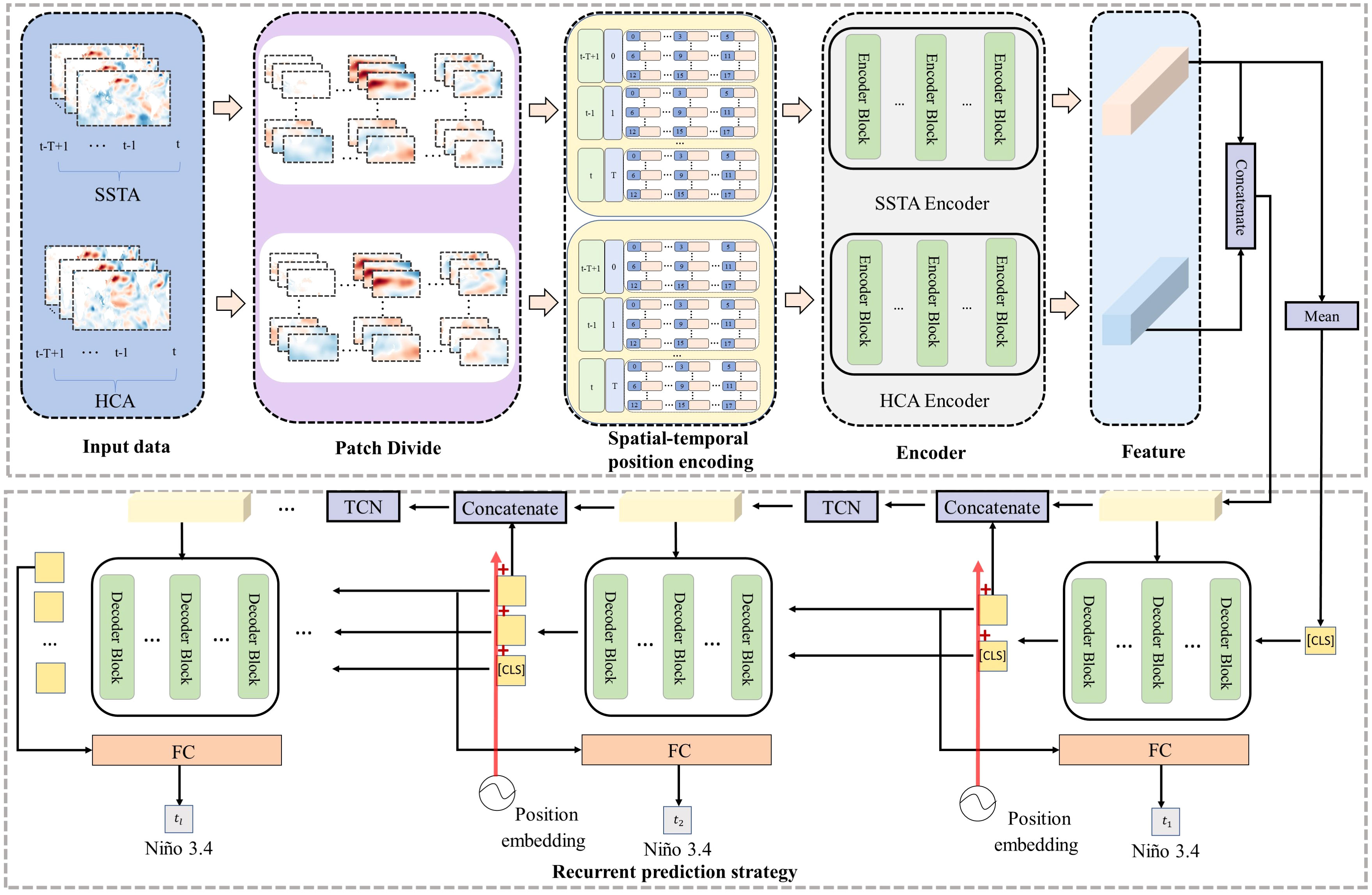
Figure 1 The proposed STTN model architecture, which contains Input data, Patch Divide, Spatial-temporal position encoding, Encoder, SSTA and HCA Features, and Recurrent prediction strategy. The SSTA and HCA encoder consist of multiple transformer encoder blocks. The Recurrent prediction strategy predicts the Niño3.4 index according to the time step. Input variables are SSTA (in units of °C) and HCA (in units of °C) from t-T+1 to t (in units of month).The STTN model outputs the Niño3.4 indexes for the next l months.

The time unit of ENSO historical input data contains T consecutive months, denoted as x_sstaϵ ℝ^T×H×W and x_hcaϵ ℝ^T×H×W for SSTA and HCA, respectively. T, H, and W indicate time, height, and width for the input data, respectively. To model the spatial and temporal correlation with a global perspective, we adopt the transformer structure as the backbone of our method. To meet the requirement of transformer structure, we first reshape the SSTA and HCA 2D data into a sequence of flattened 2D patches. Taking x_ssta as an example, each grid map is divided into N patches with same size: $x_{ssta}^{\text{'}}\in {ℝ}^{T\times N\times p_1\times p_2}$, N=H×W/(p₁×p₂). The p₁ and p₂ is the size of each patch, then each patch is converted into a one-dimensional vector with p₁×p₂ dimension. Then, we adopt a linear layer to project these vectors into D dimension. Finally, the features of the SSTA or HCA can be represented as f_ssta∈ℝ^T×N×D and f_hca∈ℝ^T×N×D .

2.2 Spatial-temporal position encoding

Due to the complex historical input data with periodic characteristics, we need to assign the position indexes for each patch to let the network know the location and order of each patch, so that the model can explore the correlations among different locations or at different times. To encode the temporal information, we adopt different sine and cosine functions Vaswani et al. (2017), which are periodic and can explore the temporal characteristic of abnormal temperature. Take f_ssta as an example:

where i is the time step of the input sequence or the calendar month in the period of C, and j is the index of dimension, PO∈ℝ^T×D . For the location of each patch within space, we learn spatial positional embedding E∈^N×D . Finally, the spatio-temporal position is added to the feature f_ssta and to obtain the embedding vector $z_{ssta}^{(0)}$.

where Norm is the LayerNorm operator, and the embedding vector $z_{hca}^{(0)}$ of HCA can also be obtained by the above process. In addition, the calendar month information and the time step of the input sequence also contributed to the recurrent prediction strategy which will be presented later.

2.3 Spatial-temporal attention module

To better model the spatial and temporal characteristics of ENSO, we adopt a multi-head attention to encode the variability. Without losing generality, we take SSTA data as the input. The encoder structure is shown in Figure 2A, which consists of spatial and temporal attention, multi-layer perceptron, and residual connection to obtain the feature representation. To capture the temporal dynamics, we first use the self-attention mechanism in the time dimension. For example, in the case of temporal attention, exclusively using keys from the same patches but different frames as the query, the query, key, and value vectors in the m-th Encoder block can be computed from the feature vector z^(m−1)∈ℝ^N×T×D as follows.

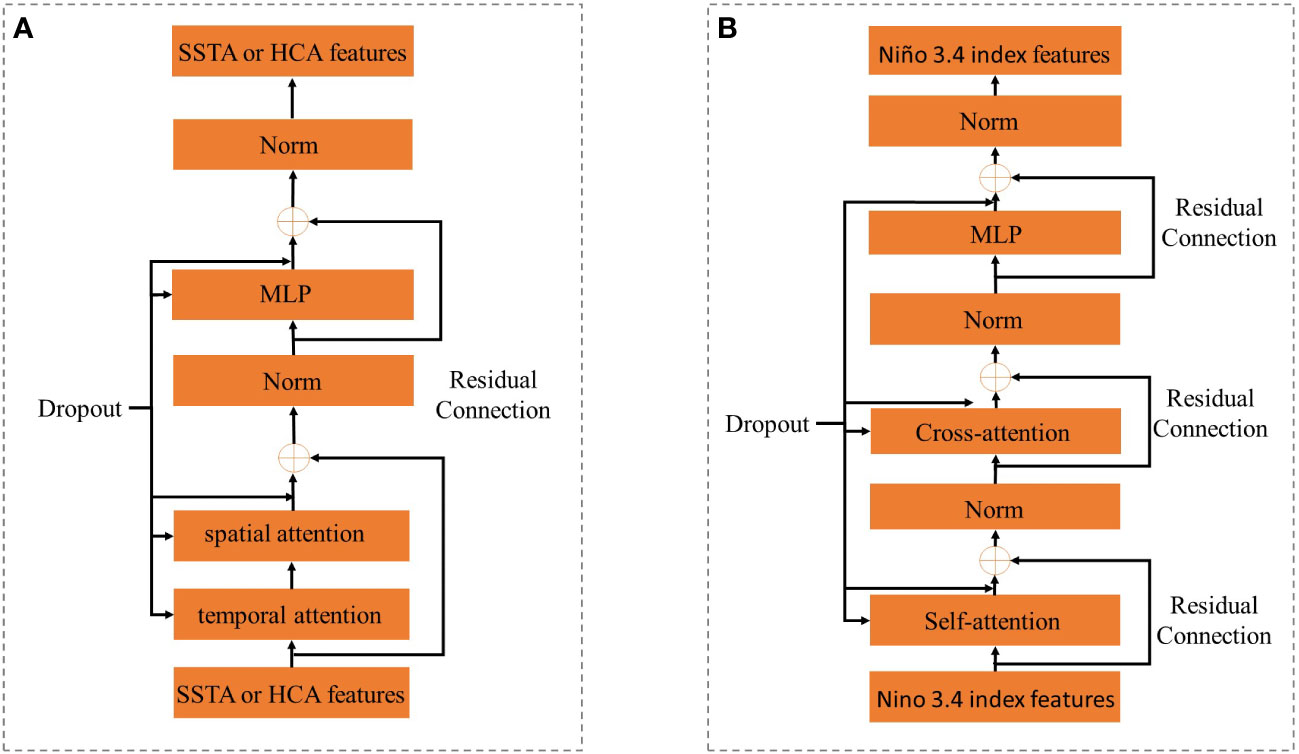
Figure 2 The Encoder and Decoder Blocks. The input to the Encoder Block is the SSTA (HCA) feature output by the upper-level block. The input to the Decoder Block is the Niño3.4 index feature output by the upper-level block.

where t = 1,…,T, and Norm is the LayerNorm operation, a = 1,…,A is the index of attention heads, and A is the sum of attention heads, the dimension of the attention head is given as D_h = D/A. $W_q^{(m,a)},W_k^{(m,a)},W_v^{(m,a)}$ are the parameters for the projection layers. The weights of temporal patches are obtained by a dot product calculation as follows.

where σ is the softmax activation function and $a_t^{(m,a)}\in {ℝ}^{T\times T}$ is the temporal attention layer m in terms of a-th head. The patch representations are calculated by these weights.

Then, these vectors from all the attention heads are concatenated and projected:

where W_t is the parameter of the linear layer and [] indicates concatenation operation. Further, to capture the spatial dynamics, we use the spatial attention immediately after the temporal attention. The spatial attention calculates the weights in the spatial dimension, exclusively using keys from the same frame as the query. When implementing the spatial attention, we can exchange the spatial and temporal dimensions of $z_t^m\in {ℝ}^{N\times T\times D}$, then the query, key, and value vectors can be computed from the feature vector $z_t^m\in {ℝ}^{T\times N\times D}$ as follows:

Then, the weight of each space patch also can be computed by the dot product calculation:

where $a_s^{(m,a)}\in {ℝ}^{N\times N}$ and σ is the softmax activation function. The encoding of the spatial attention at layer m can be similarly obtained by Eq. 6

Finally, we can also obtain the output $z_s^{(m)}$ of spatial attention as follows:

where W_p is the parameter of the linear layer and [] indicates the concatenation operation. After using the temporal and spatial attentions, we use the residual connection and multilayer perceptron (MLP) to ensure the stability of the gradient and mine the spatio-temporal features.

After encoding SSTA and HCA data, we get the spatio-temporal features of SSTA and HCA respectively, and in order to perform joint prediction, we concatenate the features of SSTA and HCA to get the feature Z∈ℝ^(2×T×N)×D .

2.4 Recurrent prediction strategy

In order to use previous predictions as prior knowledge for long-term prediction, we introduced an effective recurrent prediction strategy (RPS). Specifically, we first utilized the self-attention,cross-attention blocks, MLP layer, and residual connection to construct the decoder of the spatial-temporal characteristics. The structure of the decoder is depicted in Figure 2B. Then, the temporal convolutional block with one-dimensional convolution was adopted to encode the prediction context, which can help reduce the error accumulation in the recurrent prediction process. Finally, the fully connected layer maps the feature vector into the Niño3.4 index to optimize the whole network. It is worth noting that these operations are used in each step of the recurrent prediction. Since the Niño3.4 index is calculated by SSTA, we averaged the features of the SSTA to generate the start character CLS Vaswani et al. (2017). When predicting the Niño3.4 index for the l-th lead month, the complete calculation is as follows. First, the output of the decoder before the (l-1) th month is concatenated with CLS to generate the input e⁰∈ℝ^l×D , which is used for the decoder query. Meanwhile, the time sequence position encoding and calendar month information in the period of C are added to the output of the decoder before the concatenation, and then e⁰ is input to the decoder to predict the Niño3.4 index for the l-th lead month. The process of the decoder is shown below:

where e^m-1 is output of the m-1 layer decoder block, SA is self-attention. To prevent future information leaks, we use the mask[31] to ensure that the l-th lead month feature can only depend on known outputs smaller than the l feature location in e^m-1. CA is cross-attention, and its query/key/value can be computed by e'^(m)/Z/Z. e^m is the output of decoder for the l-th lead month, then we can get the l-th lead month Niño3.4 index after through a fully connected layer. Moreover, in order to use previous predictions as prior knowledge for long-term projection, we concatenate $e_l^m$ into the input features Z of the CA, l is an index of e^m, and use a one-dimensional convolution with k convolution kernels to mitigate the error accumulation.

3 Experiments

3.1 Dataset and Evaluation metrics

3.1.1 Dataset

Following the existing work Ham et al. (2019), we validate our proposed method on Coupled Model Intercomparison Project Phase 5 (CMIP5, details in Table 1 Ham et al. (2019)) Taylor et al. (2012), Simple Ocean Data Assimilation (SODA) Giese and Ray (2011), and Global Ocean Data Assimilation System (GODAS)Behringer and Xue (2004). These datasets contain the anomaly maps of SST and HC from 180°W-180°E and 55°S-60°N, the spatial resolution of each map is 5° x 5°. The goal of these datasets is to predict the Niño3.4 indexes in the next consecutive months. The details of the data are shown in Table 2. The training dataset includes simulated data from the CMIP5 Taylor et al. (2012) in the period from 1861 to 2004, the validation dataset includes the reanalysis data from the SODA Giese and Ray (2011) in the period from 1871 to 1973, and the test dataset includes the reanalysis data from the GODAS Behringer and Xue (2004) in the period from 1982 to 2017. All methods utilize the same data for training, validation and evaluation. In addition, following the existing work Zhou and Zhang (2022), we also validated our proposed method in Coupled Model Intercomparison Project Phase 6 (CMIP6 Eyring et al. (2016)), SODA, and GODAS. These datasets contain the anomaly maps of SST and HC from 175°W-175°E and 50°S-50°N, the spatial resolution of each map is 5° x 5°, and the details of the data are shown in Table 3. It is worth noting that the dataset in Table 3 was used only for comparison with Zhou and Zhang (2022).

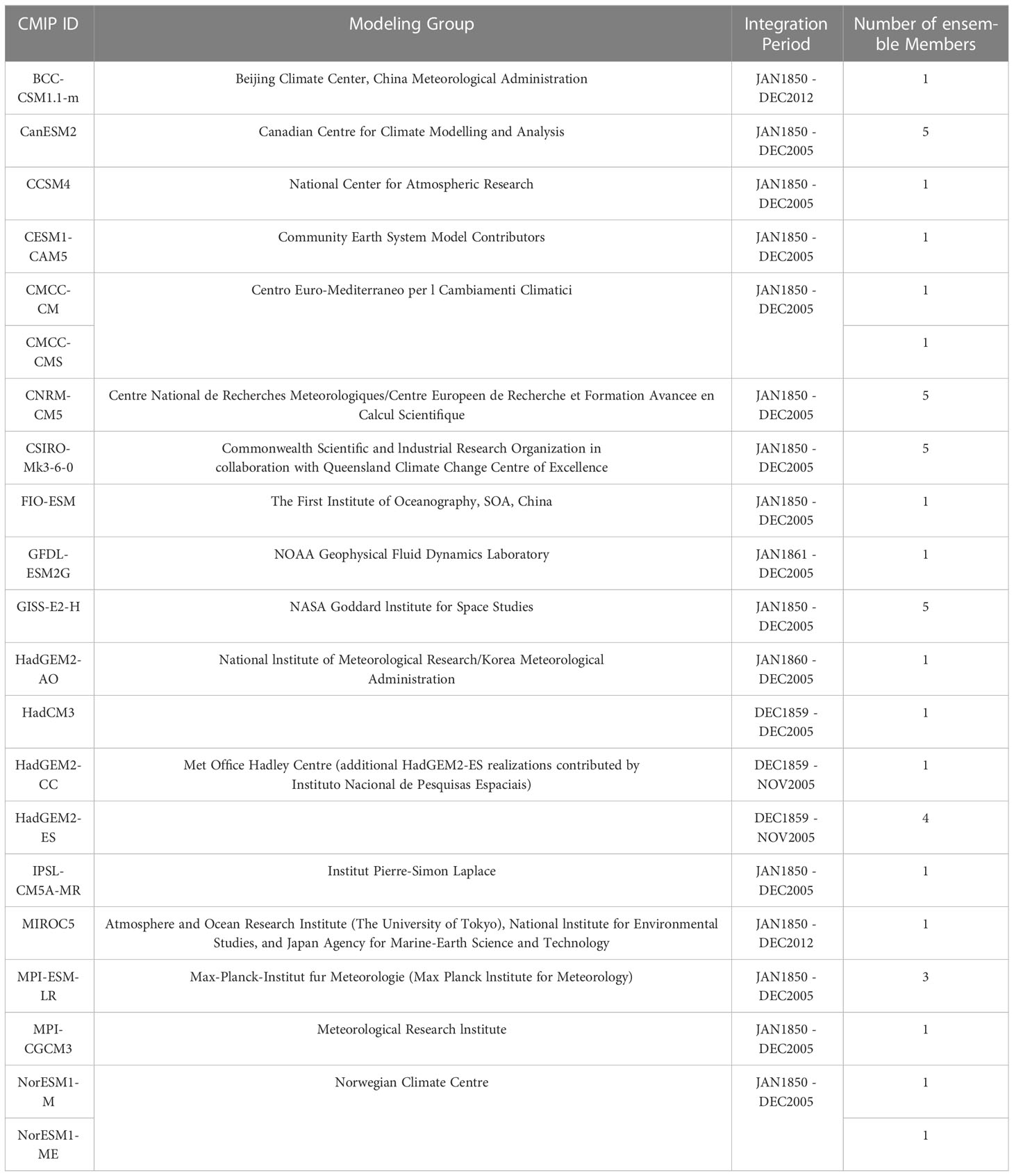
Table 1 Details of the CMIP5 models used in this study.

Table 2 The training, validation and testing subsets for Niño3.4 index prediction on CMIP5 dataset.

Table 3 The training, validation and testing subsets for Nino3.4 index prediction on CMIP6 dataset.

3.1.2 Evaluation metrics

To fairly evaluate the performances of the proposed method and competing methods, we adopted Temporal Anomaly Correlation Coefficient Skill (Corr) and Root Mean Square Error (RMSE) between the predictions and observations with different leading months l, as used in Ham et al. (2019). Corr is a measure of linear correlation between predicted and observed values, and RMSE is the standard deviation of the residuals, which is a standard measure of prediction error between predicted and observed values. In addition to the above metrics for evaluating the performance of ENSO prediction, we also calculated the Mean Absolute Error (MAE) to evaluate the average absolute values. The formulations of Corr, RMSE, and MAE are as follows:

where P is the predicted value, Y is the observed value, ${\overline{P}}_{m,l}$ is the mean of P, ${\overline{Y}}_m$ is the mean of Y, m is the calendar month, ranging from 1 to 12. s and e are the start and end years of the data, respectively.

3.1.3 Implementation details

Our approach was implemented on the Pytorch framework, and all experiments were performed on an NVIDIA RTX3090ti with 24 GB of memory. We adopted the strategy of Adaptive moment estimation (Adam) to optimize the network learning. Following the Noam Optimizer Vaswani et al. (2017), we adjusted the learning rate during training. In order to clearly understand the experimental setup, we list the main hyperparameter symbols, descriptions, and the values being set in Table 4, the B₁, B₂, $p_1^{\text{'}}$, $p_2^{\text{'}}$, p₁, p₂ are set to 160, 80, 8, 12, 10, 14, respectively. The number of layers M of Encoder and Decoder is fixed to 6, the value for attention head A is fixed to 6, and D₁ and D₂ are set to 384 and 768. The convolution kernel of the temporal convolutional network is k=4. The dropout rate d is set to 0.1. The pos in the input sequence of the Encoder is set to 0, 1, 2 and it is set to 3,…26 in the Decoder. The ENSO cycle C is set to 2. For the reproducibility of the experiments, the seeds of CPU and GPU are both 5 when we initialize the parameters, and the GPU seed is 0 when the model is training.

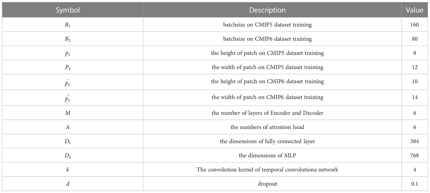
Table 4 The hyperparameter symbols, descriptions and values in this study.

3.2 Comparisons with state-of-the-arts

We compare our method with several representative methods, including numerical prediction and deep learning methods, respectively. The numerical weather prediction contains Scale Inter-action Experiment-Frontier(SINTEX-F) Luo et al. (2008) and the North American MultiModal Ensemble (NMME) Kirtman et al. (2014) with CanCM3, CanCM4, CCSM3, CCSM4, GFDL-aer04, GFDL-FLOR-A06 and GFDL-FLOR-B01. The deep learning method consists of multiple ensemble CNN Ham et al. (2019) and multi scale CNN with parallel deep network(MS-CNN) Ye et al. (2021b), and ensemble model ENSOTR Ye et al. (2021a) with Transformer module. The results are shown in Figure 3. It display the all-season Corr(ACorr) for three-month-moving-average Niño3.4 index in 1982-2017 and there are several conclusions can been observed:

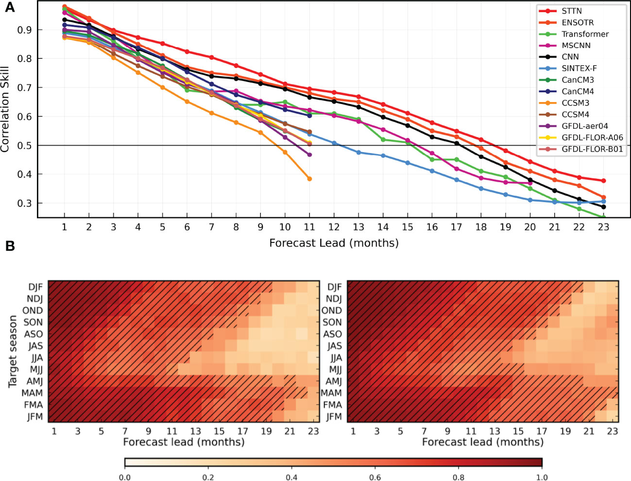
Figure 3 ENSO predicts all-season Temporal Anomaly Correlation Coefficient Skill (ACorr) in the STTN model. (A) The ACorr of the three-month-moving-averaged Nino3.4 index with Several lead times from ˜ 1982 to 2017 in the STTN model(red), Convolutional Neural Network (CNN) model (black), parallel deep CNNs with heterogeneous Architectures MS-CNN(Light purple), ENSO transformer(ENSOTR)(Orange color), Transformer(Lemon-green), Scale Interaction Experiment-Frontier dynamical prediction system (Sky blue), including additional dynamic prediction systems in the North American Multi-Modal Ensemble (NMME) project (other colors). The ACorr of the Nino3.4 index of every season in the ensemble CNN ˜ model (B.left) and the STTN model (B.right). The light black line indicates that ACorr is equal as 0.5.

3.2.1 Numerical prediction vs deep learning

All deep learning methods (e.g. CNN, MS-CNN and Transformer, etc.) outperform the numerical prediction methods (e.g. SINTEX-F and NMME). The main reason is that the numerical prediction methods design mathematical models of the atmosphere and ocean to mine complex variations with complex calculation processes, while the data-driven deep model can automatically explore the variant characteristics of the EI Niño-Southern Oscillation.

3.2.2 CNN-based method vs transformer-based method

The ACorr of single CNN model is above 0.5 for a lead of 13 month prediction Ye et al. (2021b), while the ACorr of multi-scale CNN model is above 0.5 for a lead of 15 month prediction Ye et al. (2021b), which demonstrates that different scales of convolutional kernel sizes utilize multiple receptive fields to better obtain the region correlations. Moreover, the transformer-based methods (e.g. Transformer and ENSOTR) adopt the attention mechanism to conduct spatial interactions and easily obtain global correlations between different regions and outperform the CNN-based methods.

3.2.3 Transformer-based mehtod vs ours

Our proposed method dramatically outperforms the state-of-the-art methods. Specifically, our method without using ensemble multiple models outperforms the ensemble model ENSOTR for all predicted lead months, especially for 3-10 lead months. Comparing to Transformer and ENSOTR, our method not only designs the attention mechanism across both spatial and temporal dimensions but also incorporates the knowledge of prediction and influence of seasonal variation into the learning procedure, which better facilitates the EI Niño prediction.

Figure 3B shows the Corr of the Niño3.4 index variation for each calendar month. The figure shows that our model (right) predicts more months with a Corr of the Niño3.4 index higher than 0.5. In particular, when the target season is May-June-July (MJJ), the SINTEX-F only contains 4 months Ham et al. (2019), the MS-CNN contains 10 months Ye et al. (2021b), and the CNN ensemble model (left) contains 11 months with a correlation coefficient skill higher than 0.5. Our method has 15 months for which the correlation coefficient skill is up to 0.5, which shows that our method can effectively mitigate the drifts of SST and HT due to the springtime equatorial Pacific trade winds. In summary, the ACorr of the Niño3.4 index of our model outperforms all competing methods and can skillfully predict the EI Niño3.4 index over 18 months.

3.2.4 Comparison on the CMIP6 dataset

We also compare our method with POP-Net Zhou and Zhang (2022), which is currently the best performing method trained on the CMIP6 dataset. The results are shown in Figure 4. The ACorr of POP-Net model is above 0.5 for a lead of 17 month prediction, while the ACorr of our model is above 0.5 for a lead of 18 month prediction. In general, the ENSO prediction skill of our model is better relative to POP-Net, especially when the lead month is in the range of 12-24. The main reason is that the STTN model can use previous predictions as a priori knowledge for future predictions, which can provide reliable long-term forecasts.

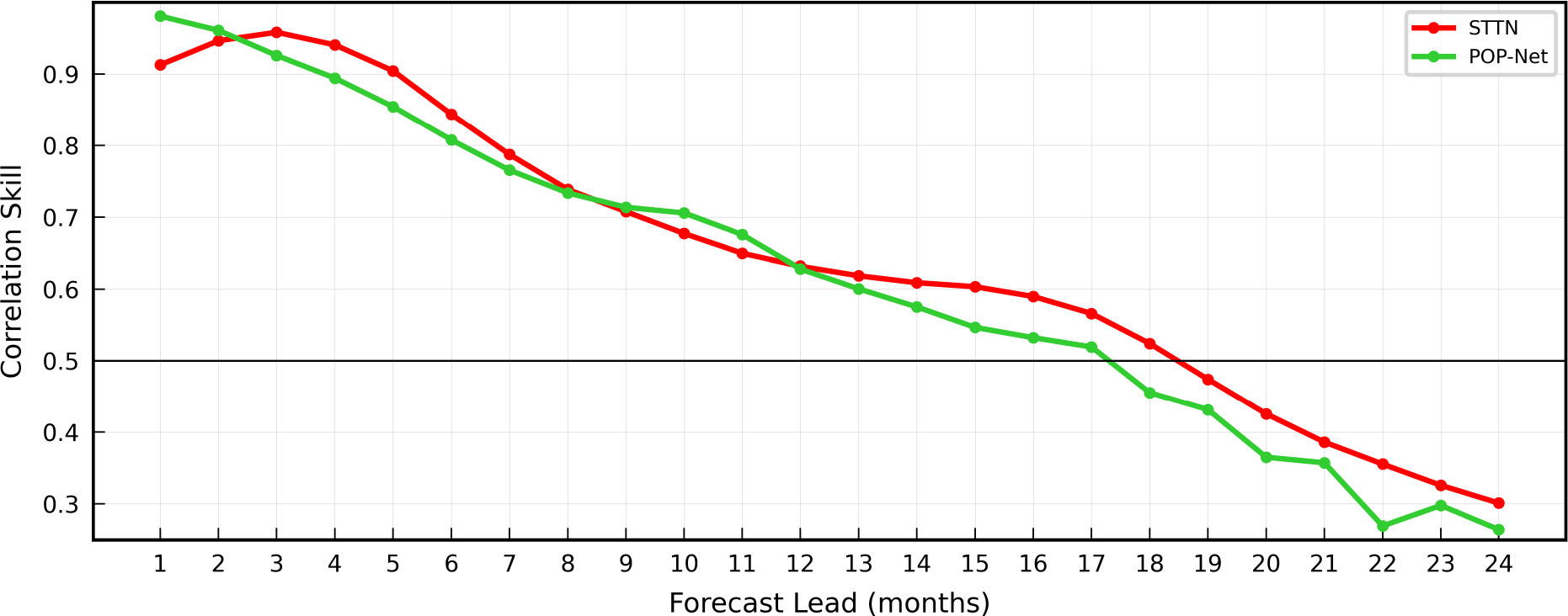
Figure 4 ENSO predicts all-season Temporal Anomaly Correlation Coefficient Skill (ACorr) in the STTN model.The ACorr of the three-month-moving-averaged Nino3.4 index index with Several lead times from ˜ 1994 to 2020 in the STTN model(red), POP-Net(Lemon-green).

3.2.5 Comparison of computational resources of different models

Table 5 compares the number of parameters and time cost for the training and testing of the CNN model Ham et al. (2019) and our model. Since the CNN model uses integrated learning, the total number of models is 11040 (23 leadmonths, 12 target months, 4 network settings, and 10 training sessions per model). The number of parameters in the four network settings is 0.12M, 0.18M, 0.21M, and 0.32M, respectively, and the total number of parameters is 2290.8M, which is much larger than our model. In addition, the training and testing time of our model is much lower than that of the CNN model, because STTN only uses the single model instead of the integrated model. The Niño 3.4 index for the next 23 lead months is available in a single run using the STTN model, which indicates that our model can predict the occurrence of El Niño in a more timely and rapid manner.

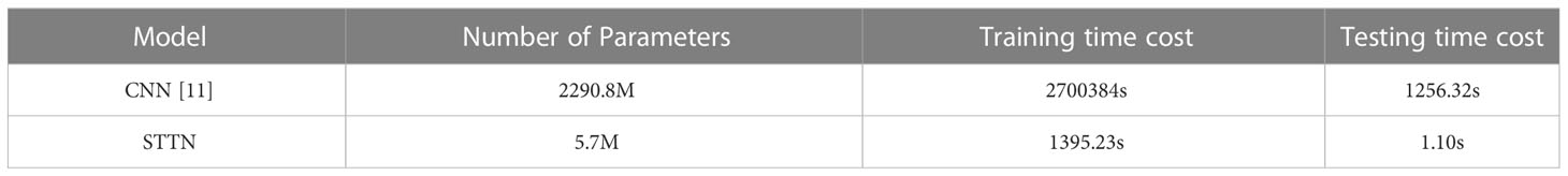
Table 5 Comparison of the computational costs required for different models.

3.3 Ablation study

In order to verify the importance of our different modules, we performed ablation experiments for each module. To keep the experiment fair, we use the same experimental setting during training as well as testing, including data partition and network hyperparameters. We remove the proposed module from the final network model STTN to demonstrate the effectiveness of using the monthly index of period, the previous prediction as prior knowledge, and TCN, respectively. W/O X indicates the removal of the X module. Figure 5 shows the ACorr, RMSR, and MAE when the monthly index of period (w/o p), previous prediction as prior knowledge (w/o F-T N), and TCN (w/o TCN) are removed, respectively. In addition, We also compared the effectiveness of spatio-temporal attention and input data of different lengths.

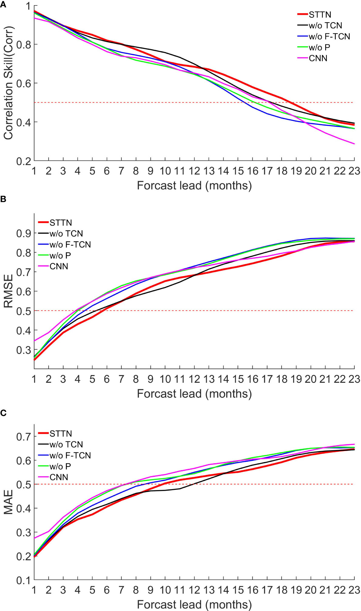
Figure 5 Comparison of (A) Corr, (B) RMSE, and (C) MAE between Niño3.4 index predictions and observations obtained with different modules. w/o X indicates removal of the X module. The purple line indicates the result of the CNN model.

3.3.1 W/o P

The overall performance of the STTN model decreased after removing the monthly index of period, which indicates that although the neural network can capture the correlation between data, it cannot capture the period of ENSO. By adding monthly indicators of periodicity, the model can be guided to effectively capture the seasonality and periodicity of the El Niño phenomenon, reducing the complexity of the model in extracting valid features from the input data and helping the model to accurately predict the Niño3.4 index.

3.3.2 W/o F-TCN

After removing the previous predictions as prior knowledge, the ACorr between the predicted and observed Niño3.4 index decreased sharply, especially in the long-term prediction, which indicates that the model does not predict the trend of evolution of El Niño over the next 23 months well when considering the input data alone. As shown in Figures 4B, C, where the MAE and RMSE increase after removing the previous prediction, it indicates that the previous predictions can compensate over long intervals and provide reliable long-term predictions.

3.3.3 W/o TCN

With the removal of the TCN module, we observed a low degradation in the performance of the model, which indicates that the cycle and future features are very important information. Compared to STTN, the model relies more on thepredicted Niño3.4 index series after lead month 12, which suggests that the temporal semantics are significant in the later stage for Niño3.4 index prediction.

3.3.4 Effectiveness of spatio-temporal attention

We compared the performance of the models using spatio-temporal attention and without using spatio-temporal attention. Figure 6A-C plots the ACorr, RMSR, and MAE of the prediction results. We first observed that the model with spatio-temporal attention performs better than the model without spatio-temporal attention. The spatio-temporal attention semantically learns more separable features and effectively reduces the spatio-temporal chaos, allowing the model to better fit the ENSO phenomenon. As can be seen from Table 6, these modules all favor ENSO prediction, and removing any of the modules would harm the performance.

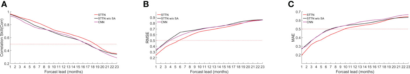
Figure 6 Comparison of (A) Corr, (B) RMSE, and (C) MAE between Niño3.4 index predictions and observations obtained using spatio-temporal attention or attention. The purple line indicates the result of the CNN model.

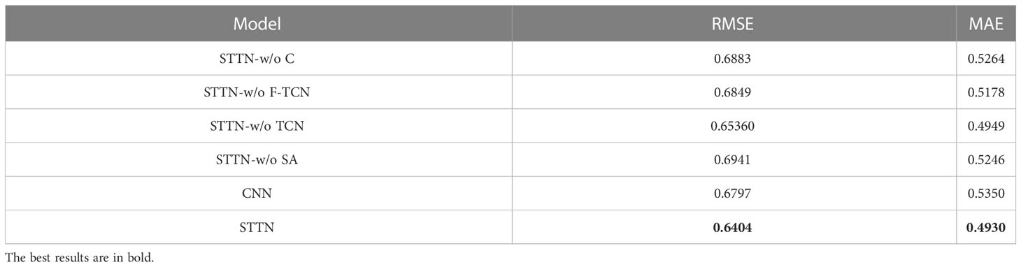
Table 6 The RMSE and MAE between Niño3.4 index predictions and observations obtained using different modules and the CNN model.

3.3.5 Compare input data of different lengths

We compared the performance of different lengths of input data. Figure 7A-C plots the ACorr, RMSR, and MAE of the predicted results. We observed that the best performance is achieved when the input data length is 3 in lead months 1-8, better performance is achieved when the input data length is 6 or 9 in lead months 8-15, and relatively better performance is achieved when the input data length is 12 in lead months 15-23, so we can conclude that: (1) the early prediction may simply require the SSTA and HCA data that are close in time to the predicted month, and the earlier month may cause noise in the input data; and (2) longer-term predictions require longer inputs, which we speculate may be due to the longer inputs containing more physical laws of ENSO as a result of the westward shift within the ocean.

Figure 7 Comparison of (A) Corr, (B) RMSE, and (C) MAE between Niño3.4 index predictions and observations for different lengths of input data. The STTN-3, STTN-6, STTN-9, STTN-12 indicate that the length of input data is 3, 6, 9, 12 months, respectively.

3.4 Case study

To clearly show the difference between the observed and predicted results from 1982 to 2017, we visualized the Niño3.4 index on the GODAS dataset for 1, 3, 6, 9, 12, and 15 lead months ahead, as shown in Figure 8. From the results, we found that the Niño3.4 indexes at 1-, 3-, 6-, and 9-lead months are accurately predicted and obtain a correlation coefficient skill of 0.97, 0.91, 0.82, and 0.74, respectively. When the lead month increased, the correlation coefficient skill decreased due to the absence of evidence for a long time series and the complex climate variation. Nonetheless, the correlation coefficient is 0.61 and over 0.5 when predicting the index for 15 lead months, which verifies the effectiveness of our method to predict the multi-year ENSO trend.

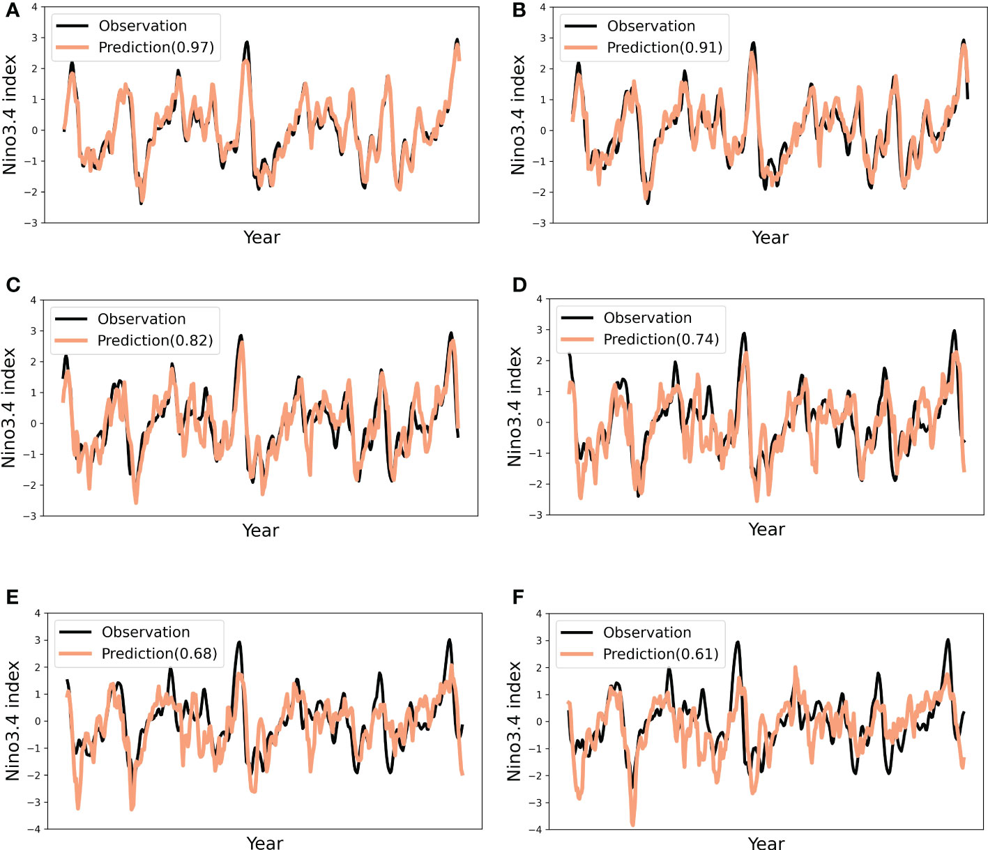
Figure 8 The Niño3.4 index of STTN model predictions and observations from 1984 to 2007 with (A) 1, (B) 3, (C) 6, (D) 9, (E) 12, and (F) 15 of lead months,respectively.

To explore the seasonal impacts, we show the predicted Niño3.4 index of averaging the December-January-February(DJF) season of 1, 6, 12 and 18 lead months in Figure 9. It can be observed that our method successfully predicts the amplitude of the Niño3.4 index at 6 lead months in advance. Even when we increase the lead time up to 18 months, the trend of our predicted results still fits the curve well when a strong El Niño or La Niña occurs. Moreover, we visualize the predicted results of a typical Super El Niño during (A) 1982-1983, and (C) 2015-2016 as well as a Super La Niña during (B) 1988-1989 in Figure 10. The predictions are the continuous outputs of our method from 1 to 23 lead months, and we can see that our model can successfully predict the evolution of these strong EI Niño phenomena and the results are consistent with the observed results even for longer lead times.

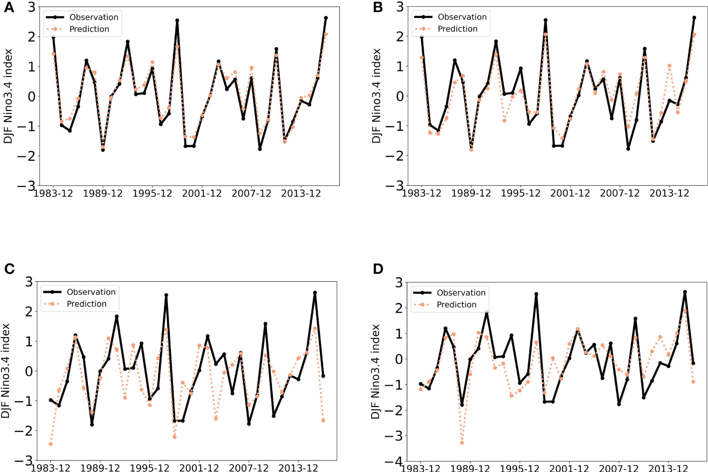
Figure 9 Predicted and observed values of Niño3.4 index for the December-January-February season, with (A) 1, (B) 6, (C) 12, (D) 18 months for lead months.

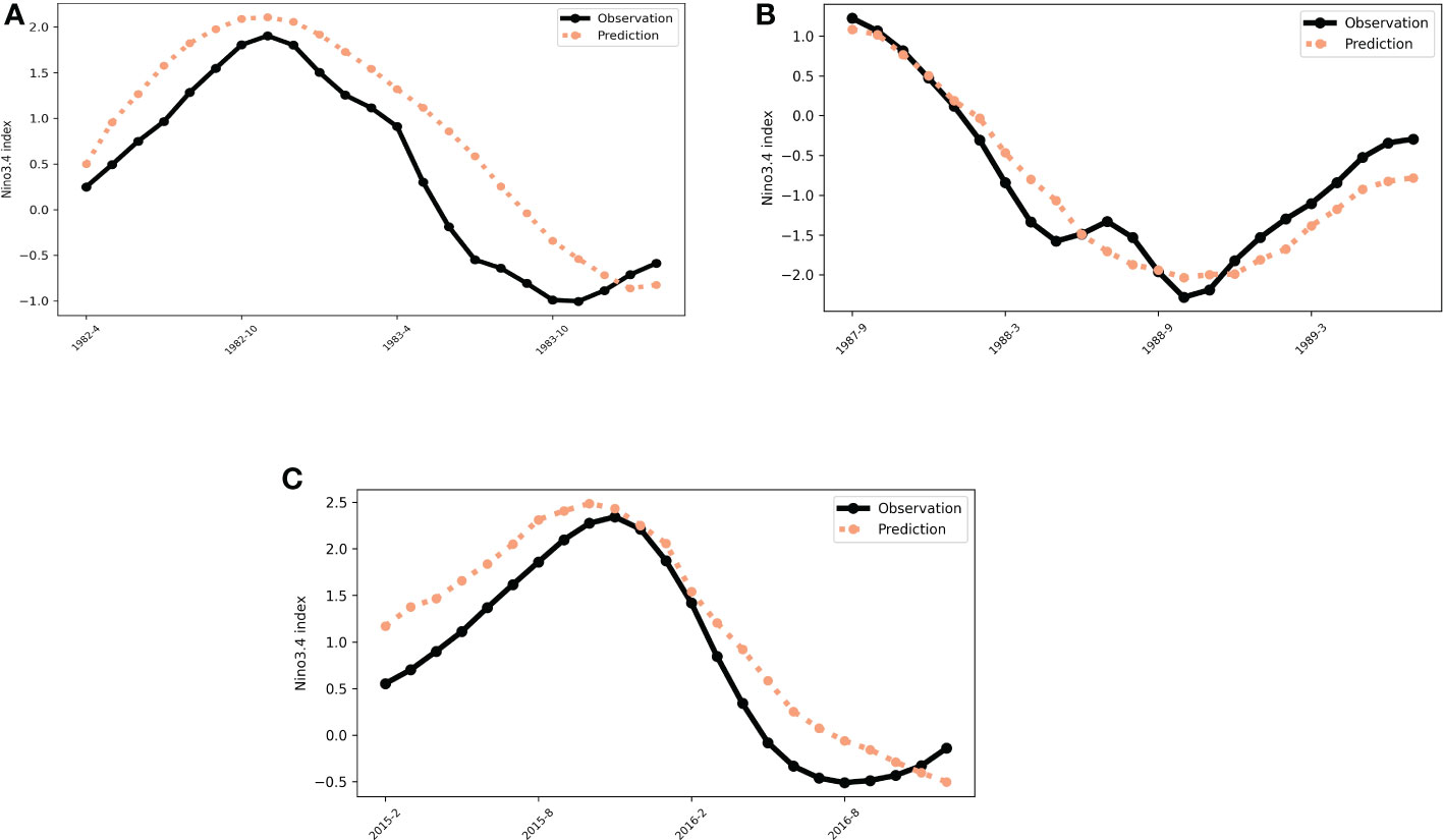
Figure 10 The 23 consecutive months output of STTN model in Super El Niño event at (A) 1982-1983, (C) 2015-2016 and Super La Nina at (B) 1988-1989.

As both the SSTA and HCA influence the ENSO phenomenon, we visualize the contributions of these two factors in Figure 11. This figure shows that when we input three consecutive months during the 1997-1998 Super El Niño event, they have different weightings to predict the Niño3.4 index in the next 23 months, which can help us understand how our method can predict El Niño for such a long time. The first row indicates the heat map of SSTA and another row indicates the heat map of HCA. Three columns indicate the time series from December 1997 to February 1998. The darker color represents the more important. From the figure we have the following observations:

● SSTA and HCA show different contributions in both the spatial and temporal dimensions. With the increasing of time, their importance in different spatial locations gradually increase.

● SSTA plays a more important role than HCA at earlier times (first two columns) in predicting the Niño3.4 index. The third column shows that the contributions of SSTA and HCA close to the predicted future are almost equal, which demonstrates that our method takes full advantage of these two inputs and their complementary relationship.

● The global heat map induces a similar observation to Ham et al. (2019) that the anomalies over the tropical western Pacific, Indian Ocean, and subtropical Atlantic are the main regions to accurately predict the 1997/98 El Niño phenomenon.

● With the change over time (from first column to third column), the contributions of the western part of the map are increasing due to the westward movement that occurs within the ocean.

Figure 11 The heat map of the contribution of SSTA (in units of °C) and HCA (in units o °C) data to the prediction of the STTN model for the 1997/1998 Super El Niño event for the following 23 consecutive months (The dashed and solid line distributions indicate negative and positive values of SST or HC anomalies). The SSTA and HCA input data are from 1997-December, 1998-January, and 1998-February, respectively.

4 Conclusion

In this paper, we propose a novel spatial-temporal transformer network for multi-year ENSO prediction. Motivated by the attention mechanism, we designed a spatial-temporal attention mechanism to model the contributions of different ocean locations with change over time. For long-term prediction, this article proposes utilizing the accurate previous prediction as prior knowledge and fusing the seasonal variation during the encoding of the temporal information to facilitate the ENSO prediction. Moreover, we use a single model instead of a multi-model architecture to reduce computational resources, which is more convenient for predicting ENSO with different lead times. Extensive experiments using the model on the Coupled Model Intercomparison Project phase 5 (CMIP5) and the Coupled Model Intercomparison Project phase 6 (CMIP6) have shown that our method can provide a more accurate prediction over the existing methods, which verifies the effectiveness of the spatial-temporal attention mechanism, the prior knowledge of previous prediction and the temporal index for modeling the seasonal variation. In the future, we will add more variables and fully explore the relationship among their sea-air interactions to facilitate the reliability of multi-year ENSO prediction.

Data availability statement

Publicly available datasets were analyzed in this study. This data can be found here: https://doi.org/10.5281/zenodo.3244463.

Author contributions

DS contributed to conceptualization and editing, and supervision. XS data processing, modeling, and writing of the original draft. WLi performed methodology and writing review, A-AL performed validation and review. TR and WLiu, performed validation and investigation. ZS optimized the model framework. All authors contributed to the article and approved the submitted version.

Funding

This work was supported in part by the National Key Research and Development Program of China (2021YFF0704000) and the National Natural Science Foundation of China (U22A2068).

Conflict of interest

The authors declare that the research was conducted in the absence of any commercial or financial relationships that could be construed as a potential conflict of interest.

Publisher’s note

All claims expressed in this article are solely those of the authors and do not necessarily represent those of their affiliated organizations, or those of the publisher, the editors and the reviewers. Any product that may be evaluated in this article, or claim that may be made by its manufacturer, is not guaranteed or endorsed by the publisher.

References

Alexander M. A., Bladé I., Newman M., Lanzante J. R., Lau N.-C., Scott J. D. (2002). The atmospheric bridge: The influence of enso teleconnections on air–sea interaction over the global oceans. J. Climate 15, 2205–2231. doi: 10.1175/1520-0442(2002)015<2205:TABTIO>2.0.CO;2
Barnston A. G., Tippett M. K., Ranganathan M., L’Heureux M. L. (2019). Deterministic skill of enso predictions from the north american multimodel ensemble. Climate Dynamics 53, 7215–7234. doi: 10.1007/s00382-017-3603-3
Bauer P., Thorpe A., Brunet G. (2015). The quiet revolution of numerical weather prediction. Nature 525, 47–55. doi: 10.1038/nature14956
Behringer D., Xue Y. (2004). Eighth symposium on integrated observing and assimilation systems for atmosphere, oceans, and land surface. AMS 84th Annual Meeting Seattle, Washington: Washington State Convention and Trade Center, 11–15.
Broni-Bedaiko C., Katsriku F. A., Unemi T., Atsumi M., Abdulai J.-D., Shinomiya N., et al. (2019). El Niño-southern oscillation forecasting using complex networks analysis of lstm neural networks. Artif. Life Robot 24, 445–451. doi: 10.1007/s10015-019-00540-2
Cachay S. R., Erickson E., Bucker A. F. C., Pokropek E., Potosnak W., Osei S., et al. (2020). Graph neural networks for improved el n/no forecasting. doi: 10.48550/arXiv.2012.01598
Eyring V., Bony S., Meehl G. A., Senior C. A., Stevens B., Stouffer R. J., et al. (2016). Overview of the coupled model intercomparison project phase 6 (cmip6) experimental design and organization. Geosci. Model. Dev. 9, 1937–1958. doi: 10.5194/gmd-9-1937-2016
Feng Q. Y., Vasile R., Segond M., Gozolchiani A., Wang Y., Abel M., et al. (2016). Climatelearn: A machine-learning approach for climate prediction using network measures. Geosci. Model. Dev. Discussions, 1–18. doi: 10.5194/gmd-2015-273
Giese B. S., Ray S. (2011). El Niño variability in simple ocean data assimilation (soda), 1871–2008. J. Geophysical Res.: Oceans 116. doi: 10.1029/2010JC006695
Gupta M., Kodamana H., Sandeep S. (2022). Prediction of enso beyond spring predictability barrier using deep convolutional lstm networks. IEEE Geosci. Remote Sens. Lett. 19, 1–5. doi: 10.1109/LGRS.2020.3032353
Ham Y.-G., Kim J.-H., Luo J.-J. (2019). Deep learning for multi-year enso forecasts. Nature 573, 568–572. doi: 10.1038/s41586-019-1559-7
He D., Lin P., Liu H., Ding L., Jiang J. (2019). A deep learning enso forecasting model[C]//PRICAI 2019: Trends in Artificial Intelligence. 16th Pacific Rim International Conference on Artificial Intelligence, August 26–30, 2019, Proceedings, Part II 16. (Cuvu, Yanuca Island, Fiji: Springer International Publishing), 12–23.
Johnson S. J., Stockdale T. N., Ferranti L., Balmaseda M. A., Molteni F., Magnusson L., et al. (2019). Seas5: the new ecmwf seasonal forecast system. Geosci. Model. Dev. 12, 1087–1117. doi: 10.5194/gmd-12-1087-2019
Kirtman B. P., Min D., Infanti J. M., Kinter J. L., Paolino D. A., Zhang Q., et al. (2014). The north american multimodel ensemble: phase-1 seasonal-to-interannual prediction; phase-2 toward developing intraseasonal prediction. Bull. Am. Meteorol. Soc. 95, 585–601. doi: 10.1175/BAMS-D-12-00050.1
Larkin N. K., Harrison D. (2002). Enso warm (el niño) and cold (la niña) event life cycles: Ocean surface anomaly patterns, their symmetries, asymmetries, and implications. J. Climate 15, 1118–1140. doi: 10.1175/1520-0442(2002)015<1118:EWENOA>2.0.CO;2
Li Y., Huang W., Lyu X., Liu S., Zhao Z., Ren P. (2022). An adversarial learning approach to forecasted wind field correction with an application to oil spill drift prediction. Int. J. Appl. Earth Observation Geoinform. 112, 102924. doi: 10.1016/j.jag.2022.102924
Ludescher J., Martin M., Boers N., Bunde A., Ciemer C., Fan J., et al. (2021). Network-based forecasting of climate phenomena. Proc. Natl. Acad. Sci. 118, e1922872118. doi: 10.1073/pnas.1922872118
Luo J.-J., Masson S., Behera S. K., Yamagata T. (2008). Extended enso predictions using a fully coupled ocean–atmosphere model. J. Climate 21, 84–93. doi: 10.1175/2007JCLI1412.1
Lv Z., Huang X., Cao W. (2022). An improved gan with transformers for pedestrian trajectory prediction models. Int. J. Intelligent Syst. 37, 4417–4436. doi: 10.1002/int.22724
McPhaden M. J., Zebiak S. E., Glantz M. H. (2006). Enso as an integrating concept in earth science. science 314, 1740–1745. doi: 10.1126/science.1132588
Mu B., Peng C., Yuan S., Chen L. (2019). ENSO Forecasting over multiple time horizons using ConvLSTM network and rolling mechanism. (Budapest, Hungary: International Joint Conference on Neural Networks (IJCNN). 1–8. doi: 10.1109/IJCNN.2019.8851967
Nie J., Huang L., Wang Z., Sun Z., Zhong G., Wang X., et al. (2022). Marine oriented multimodal intelligent computing: challenges, progress and prospects (in chinese). J. Image Graphics 27, 2589–2610. doi: 10.11834/jig.211267
Patil K., Doi T., Oettli P., Jayanthi V. R., Behera S. (2021). AGU Fall Meeting 2021, (New Orleans, LA.), A13I–A108.
Petrova D., Ballester J., Koopman S. J., Rodó X. (2020). Multiyear statistical prediction of enso enhanced by the tropical pacific observing system. J. Climate 33, 163–174. doi: 10.1175/JCLI-D-18-0877.1
Petrova D., Koopman S. J., Ballester J., Rodó X. (2017). Improving the long-lead predictability of el niño using a novel forecasting scheme based on a dynamic components model. Climate Dynamics 48, 1249–1276. doi: 10.1007/s00382-016-3139-y
Ren H.-L., Zuo J., Deng Y. (2019). Statistical predictability of niño indices for two types of enso. Climate Dynamics 52, 5361–5382. doi: 10.1007/s00382-018-4453-3
Reyes-Gomez V., Díaz S., Brito-Castillo L., Núñez-López D. (2013). Enso drought effects and their impact in the ecology and economy of the state of chihuahua, mexico. WIT Trans. State-of-the-art Sci. Eng. 64. doi: 10.2495/978-1-84564-756-8/007
Rosmiati R., Liliasari S., Tjasyono B., Ramalis T. (2021). Development of arima technique in determining the ocean climate prediction skills for pre-service teacher. Journal of physics: Conference series, vol. 1731. (Bengkulu, Indonesia: Mathematics and Science Education International Seminar (MASEIS)), 012072.
Solow A. R., Adams R. F., Bryant K. J., Legler D. M., O’brien J. J., McCarl B. A., et al. (1998). The value of improved enso prediction to us agriculture. Climatic Change 39, 47–60. doi: 10.1023/A:1005342500057
Taylor K. E., Stouffer R. J., Meehl G. A. (2012). An overview of cmip5 and the experiment design. Bull. Am. Meteorol. Soc. 93, 485–498. doi: 10.1175/BAMS-D-11-00094.1
Vaswani A., Shazeer N., Parmar N., Uszkoreit J., Jones L., Gomez A. N., et al. (2017). Attention is all you need. Adv. Neural Inf. Process. Syst. 30. doi: 10.1145/3295222.3295349
Wang X., Slawinska J., Giannakis D. (2020). Extended-range statistical enso prediction through operator-theoretic techniques for nonlinear dynamics. Sci. Rep. 10, 1–15. doi: 10.1038/s41598-020-59128-7
Yan J., Mu L., Wang L., Ranjan R., Zomaya A. Y. (2020). Temporal convolutional networks for the advance prediction of enso. Sci. Rep. 10, 1–15. doi: 10.1038/s41598-020-65070-5
Ye F., Hu J., Huang T.-Q., You L.-J., Weng B., Gao J.-Y. (2021a). Transformer for ei niño-southern oscillation prediction. IEEE Geosci. Remote Sens. Lett. 19, 1–5. doi: 10.1109/LGRS.2021.3100485
Ye M., Nie J., Liu A., Wang Z., Huang L., Tian H., et al. (2021b). Multi-year enso forecasts using parallel convolutional neural networks with heterogeneous architecture. Front. Mar. Sci. 1092. doi: 10.3389/fmars.2021.717184
Zebiak S. E., Cane M. A. (1987). A model el niñ–southern oscillation. Monthly Weather Rev. 115, 2262–2278. doi: 10.1175/1520-0493(1987)115<2262:AMENO>2.0.CO;2
Zhang R.-H., Gao C. (2016). The iocas intermediate coupled model (iocas icm) and its real-time predictions of the 2015–2016 el niño event. Sci. Bull. 61, 1061–1070. doi: 10.1007/s11434-016-1064-4
Zhao J., Luo H., Sang W., Sun K. (2022). Spatiotemporal semantic network for enso forecasting over long time horizon. Appl. Intell. 53, 6464–6480. doi: 10.1007/s10489-022-03861-1
Keywords: EI Niño southern oscillation, long-term prediction, spatio-temporal modeling, transformer, deep learning
Citation: Song D, Su X, Li W, Sun Z, Ren T, Liu W and Liu A-A (2023) Spatial-temporal transformer network for multi-year ENSO prediction. Front. Mar. Sci. 10:1143499. doi: 10.3389/fmars.2023.1143499
Received: 13 January 2023; Accepted: 20 February 2023;
Published: 13 March 2023.
Edited by:
Haiyong Zheng, Ocean University of China, ChinaReviewed by:
Peng Ren, China University of Petroleum (East China), ChinaZhenya Song, Ministry of Natural Resources, China
Copyright © 2023 Song, Su, Li, Sun, Ren, Liu and Liu. This is an open-access article distributed under the terms of the Creative Commons Attribution License (CC BY). The use, distribution or reproduction in other forums is permitted, provided the original author(s) and the copyright owner(s) are credited and that the original publication in this journal is cited, in accordance with accepted academic practice. No use, distribution or reproduction is permitted which does not comply with these terms.
*Correspondence: Wenhui Li, liwenhui@tju.edu.cn; An-An Liu, anan0422@gmail.com