

Abstract
The climate system is gaining heat owing to increasing concentration of greenhouse gases due to human activities. As the world's oceans are the dominant reservoir of heat in the climate system, an accurate estimation of the ocean heat content change is essential to quantify the Earth's energy budget and global mean sea level rise. Based on the mean estimate of the three Argo gridded products considered, we provide a decadal ocean heat content estimate (over 2005–2014), down to 2000 m, of 0.76 ± 0.14 W m−2 and its spatial pattern since 2005 with unprecedented data coverage. We find that the southern hemisphere explains 90% of the net ocean heat uptake located around 40°S mainly for the Indian and Pacific oceans that corresponds to the center of their subtropical gyres. We find that this rapid upper ocean warming is linked to a poleward shift of mean wind stress curl enhancing Ekman pumping for the 45°S–60°S band. Therefore, the increase of Ekman pumping steepens the isopycnal surface and can enhance heat penetration into the deeper layers of the ocean. We also highlight a relative consistency between the year-to-year net top-of-the-atmosphere flux inferred by satellite measurements and the ocean heating rates (correlation coefficient of 0.53). We conclude that there is no strong evidence of missing energy in the climate system because of remaining large uncertainties in the observing system.
Export citation and abstract BibTeX RIS

Original content from this work may be used under the terms of the Creative Commons Attribution 3.0 licence. Any further distribution of this work must maintain attribution to the author(s) and the title of the work, journal citation and DOI.
1. Introduction
In an equilibrium climate and at global scale, the absorbed solar radiation is balanced by the outgoing long wave radiation. This balance is known as the Earth's energy budget. Any perturbation of this budget will lead to an Earth's energy imbalance (von Schuckmann et al 2016). The Earth's energy imbalance is one of the best metrics to determine the actual global warming (Von Schuckmann et al 2016). It is now well established that Earth is storing thermal energy due to human activities associated with increasing concentrations of greenhouse gases into the atmosphere (Levitus et al 2001, Hansen et al 2005, Abraham et al 2013). The net top-of-the-atmosphere (TOA) energy budget experiences a recent imbalance and is best assessed by estimating changes of climate reservoirs. The world's oceans are the dominant reservoir of heat in the climate system. In fact, the oceans can store large amount of heat because of their huge mass and the important heat capacity of seawater. It has been suggested that the global ocean explains >90% of the net Earth's energy imbalance over 1971–2010 (Rhein et al 2013). Moreover, recent studies suggest that the net Earth's energy budget presents interannual to decadal variability strongly correlated with the ocean heat content (OHC) variations (Allan et al 2014, Smith et al 2015). While the precise magnitude of Earth's energy imbalance remains unclear, the interannual variability seems to be linked to natural variability such as volcano activity and El Niño/Southern Oscillation (Allan et al 2014). Therefore, as the world's oceans play a significant role in storing heat, an accurate quantification of the OHC change is essential to quantify with high accuracy the net Earth's energy imbalance.
However, estimating the net Earth's energy imbalance is not an easy task and different methods have been carried out for this purpose. One way to assess the OHC is to take advantage of climate models. Recent studies have highlighted the contribution of ocean in Earth's energy budget (Palmer and McNeall 2014) and especially the importance of deep ocean contribution (Palmer et al 2011) to evaluate and constrain the decadal OHC changes. Another possible way to assess the OHC is to consider hydrographic in situ measurements. Unfortunately, the coverage of in situ temperature measurements for the 20th century is spatially and temporally sparse, especially south of 40°S (Abraham et al 2013, Lyman and Johnson 2014), making a precise quantification of OHC changes difficult. Ship-based in situ expendable bathythermograph (XBT) measurements are the largest source of available data since the 1970s sampling mainly the upper ocean above 400 m and 700 m. Note that in situ temperature measurements sampling the upper 700 m of the global ocean represent only 20% of its net volume (Abraham et al 2013). The upper OHC change has been estimated to range between 0.22–0.27 W.m−2 over 1970–2012 (Abraham et al 2013). From 1993 to 2008, Johnson et al (2013) estimated the OHC change to be 0.51 ± 0.09 W.m−2 that is higher than the previous decades. Furthermore, the last IPCC-AR5 report states that oceans warmed with an average heating range of 0.71 W.m−2 for 1993–2010. These recent results highlight the importance of multidecadal/interannual variability of OHC changes and the need to assess with high accuracy the OHC change to establish the Earth's energy budget properly.
Since the beginning of the 2000s, the International Argo program provides indispensable temperature and salinity measurements to investigate the ocean heat content changes (Gould et al 2004). Each float records a temperature/salinity (T/S) profile of the water column every 10 days. Even if the temperature change remains small for the deeper oceanic layers compared to the upper ocean, their contributions might be significant regarding their large mass (Abraham et al 2013, Rhein et al 2013). Several studies investigated the OHC change and its contribution to the Earth's energy budget over the recent few years (Roemmich and Gilson 2009, Loeb et al 2012, Llovel et al 2014, Lyman and Johnson 2014, von Schuckmann et al 2014, Roemmich et al 2015, Wijfells et al 2016 that is an update of the work of Roemmich et al 2015) but few of them provided a decadal estimate of OHC change from the surface to 2000 m depth. Furthermore, Argo float coverage has reached a near global coverage since 2005 providing us the opportunity to investigate a decadal OHC change (with an unprecedented large amount of in situ measurements) and its contribution to the Earth's energy imbalance. Note that the ocean layers above 2000 m represent roughly 50% of the net ocean volume (Abraham et al 2013). Studies have suggested that the deep ocean (below 2000 m) would have experienced a slight warming over multidecadal time scales (Purkey and Johnson 2010, Kouketsu et al 2011). Purkey and Johnson (2010) report a slight deep ocean warming of 0.068 ± 0.061 W.m−2 over the 1990s and 2010s based on high-quality temperature data mostly from ship-based conductivity-temperature-depth (CTD) instruments. However, these studies rely on sparse observations both in space and time.
In addition, as global oceans warm, seawater expands leading to an increase of global mean sea level (Church et al 2013). This contribution is known as thermal expansion. A description on the calculation can be found in Llovel et al (2010, 2013). A recent review revisits the global mean sea level budget over 1972–2008 (Church et al 2011). The authors estimate that the thermal expansion explains 40% and 30% of the net global mean sea level rise over 1972–2008 and 1993–2008, respectively, denoting the existence of decadal variability in ocean warming. Recently, this contribution has been estimated to be one third of the net global mean sea level rise inferred by satellite altimetry over 2005–2013 (Llovel et al 2014). Therefore, a precise quantification of ocean warming is important to constrain the global mean sea level rise.
In this paper, we investigate the OHC change, its spatial pattern from January 2005 to December 2014 (10 years) and its relationship to the net top-of-the-atmosphere energy imbalance. This study aims to compliment the recent study by Roemmich et al (2015) who investigated the ocean heat content change over a shorter time period, 2006–2013, and its spatial structure using different mapping methods. In this study, we consider three Argo-based gridded products computed by different research groups that provide us the opportunity to discuss the consistency of the results. We also go a step farther by investigating the cause of such a rapid upper ocean warming by analyzing the respective contribution of surface atmospheric fluxes such as wind stress and net surface heat flux. We focus our analysis on the upper ocean warming detected in the south-east Indian and south Pacific oceans. Afterward, we present different and complementary analysis to support our findings especially with respect to the net TOA budget.
The paper is structured as follows. In section 2, we describe the data and the methods used in this study. In section 3, we present our results on the OHC change and its structure for the last decade between 2005–2014. We investigate the wind stress and surface heat flux contributions to the upper ocean warming located in the south-east Indian and Pacific oceans over the past decade. We also present the OHC contribution to the Earth's energy budget deduced from satellite measurements. Finally, in section 4, we summarize the results, address the broader implications of our findings and discuss the future work motivated by this study.
2. Data and methods
2.1. Temperature and salinity gridded products
We consider the T/S gridded products from Argo floats produced by the Scripps Institution of Oceanography (SCRIPPS, updated from Roemmich and Gilson 2009), the International Pacific Research Center (IPRC) and the Japan Agency for Marine-Earth Science and Technology (JAMSTEC, updated from Hosoda et al 2008) available at http://argo.ucsd.edu/Gridded_fields.html. Argo-based T/S profiles have been passed through meticulous quality control processes (Argo data management 2011, Wong et al 2015). There are two different quality control processes applied to each Argo float. When the Argo float transfers data at the surface, an automatically quality control is processed as quickly as possible (typically within 24 h). This first quality control test involves many checks including the platform identification, date test, the location of the float, the drift speed of the float, global or regional range tests (on temperature and salinity), pressure test, spike test, density inversion, grey list test (sensor that is not working correctly), gross salinity or temperature sensor drift and frozen profile test (see Wong et al 2015 for more information). The first step of quality control produce the real-time data. Thereafter, other procedures to check data quality are applied before returning the data to the global data center typically within 6–12 months. An operator should examine profile data for pointwise errors (mainly sensor drifts). This second quality control test is applied on pressure, temperature and salinity. This second quality control check produces the delayed mode data.
We compute the OHC time series from the surface to 2000 m depth at monthly interval on a 1° × 1° regular grid from January 2005 to December 2014 with respect to the monthly climatology (defined as the mean estimate for each calendar month) using the equation of state of seawater TEOS10 (http://teos-10.org/index.htm) at each standard level. To examine the robustness of the ocean heat content evolution, we consider 3 Argo-based gridded datasets produced by different research centers.
We compute linear trend estimates using a least square fit analysis and its uncertainty at 1-sigma based on the model misfit for the individual Argo gridded fields. For the mean estimate, we perform a weighted least squares fit at a monthly basis where the weights are chosen to equal the reciprocal variance of the three Argo gridded fields and its uncertainty at 1-sigma that includes the model misfit and the spread between the different Argo products. Regarding the figures, the grey envelopes denote the spread around the mean for the three Argo-based gridded products. We always adopt these conventions unless otherwise stated.
2.2. Surface forcing products
Wind-driven Ekman pumping causes heaving movements of the subsurface pycnoclines leading to upper ocean temperature and salinity changes whereas surface heat fluxes affect upper ocean temperature change inducing ocean heat content change. Change in wind is associated with heat redistribution although net surface heat flux modifies the localized integrated heat content. To diagnose the roles of surface forcing on the regional ocean heat content variations, we focus our analyses on wind-driven Ekman pumping and surface heat flux. The wind stress components and surface heat fluxes are obtained from the ERA-Interim atmospheric reanalysis (produced by the European Centre for Medium-Range Weather Forecast; Dee et al 2011) and National Centers for Environmental Prediction (NCEP, Kalnay et al 1996) and Modern-Era Retrospective Analysis for Research and Applications (MERRA, Rienecker et al 2011) and the Japanese 55-year Reanalysis (JRA-55, Kobayashi et al 2015). The atmospheric reanalysis provide data on a 1.5° × 1.5°, 1.875° × 1.9°, 0.5° × 0.66° and 1.25° × 1.25° global grids, respectively. In each case, we consider the monthly mean estimates from January 2005 to December 2014.
Ekman pumping velocity is defined by

Where  represents the Ekman pumping, f is the Coriolis parameter, τ is the wind stress and
  is the mean density of seawater (the seawater density has been computed with Argo-based T/S gridded data for each month over 2005–2014 with the SCRIPPS gridded product). Atmospheric flux uncertainties denote the spread around the mean based on the four atmospheric reanalysis unless otherwise stated.
2.3. Net top-of-the-atmosphere (TOA) flux data
We consider global net TOA flux data coming from CERES from January 2005 to December 2014 downloaded at http://ceres.larc.nasa.gov/order_data.php. The time series is provided at monthly average and we consider the all-sky conditions. We use the 'Energy Balanced and Filled' (EBAF) updated to version Ed2.8 (updated from Loeb et al 2012) which is constrained to an estimate of ocean heat storage term. Because we are focusing our analysis on interannual time scales, we remove the monthly mean climatology for each time series defined as the mean of each calendar month computed over 2005–2014.
We compute the ocean heating rates from the OHC time series using a centered differencing method. For the first and last values, we use a one-side differencing method instead. Because the oceans have stored more than 90% of the Earth's energy imbalance over 1970–2010 (Rhein et al 2013, Palmer and McNeall 2014), the net TOA flux and the ocean heating rates should be in phase with each other at global scale (Loeb et al 2012). Therefore, we compute the ocean heat content yearly mean average to compare directly with the net TOA flux time series.
3. Results
3.1. Ocean heat content estimate
Figure 1(a) shows the global OHC time series computed from the surface to 2000 m depth based on SCRIPPS (blue curve), IPRC (red curve), JAMSTEC (green curve) and the mean estimate (black curve). The three datasets show global OHC increase for the recent decade. However, we note some spread around the mean between the Argo gridded products especially around 2007 and 2012. The global OHC trend accounts for 8.41 ± 1.56 × 10²¹ J.yr−1 (based on the mean estimate between the three Argo products) ranging from 7.19 ± 0.5 × 10²¹ (SCRIPPS) to 10.18 ± 0.38 × 10²¹ J.yr−1 (JAMSTEC) depending on the considered dataset. In terms of equivalent planetary heating rates, the values range from 0.65 ± 0.05 W.m−2 to 0.92 ± 0.04 W.m−2 with the mean estimate of 0.76 ± 0.14 W.m−2 over 2005–2014 (per unit of the ocean surface of 350.1012 m2; table 1 summarizes the OHC trend estimates). The mean planetary heating rate is estimated from the mean ocean heat content changes of the three Argo-based gridded products. (cf, the black curve of figure 1(a)). Furthermore, we find correlation coefficients of 0.91, 0.85 and 0.93 between the OHC time series based on SCRIPPS, versus IPRC, SCRIPPS versus JAMSTEC and IPRC versus JAMSTEC, respectively. Table 1 also includes trend estimates over 2006–2013 (same period than Roemmich et al 2015). The quoted values are always smaller than our decadal estimates. This highlights the importance of interannual variability and thus, the importance of the considered time period. It is important to note that evaluating trends on a decadal time series does not necessarily represent the long-term change but the interannual variability instead.
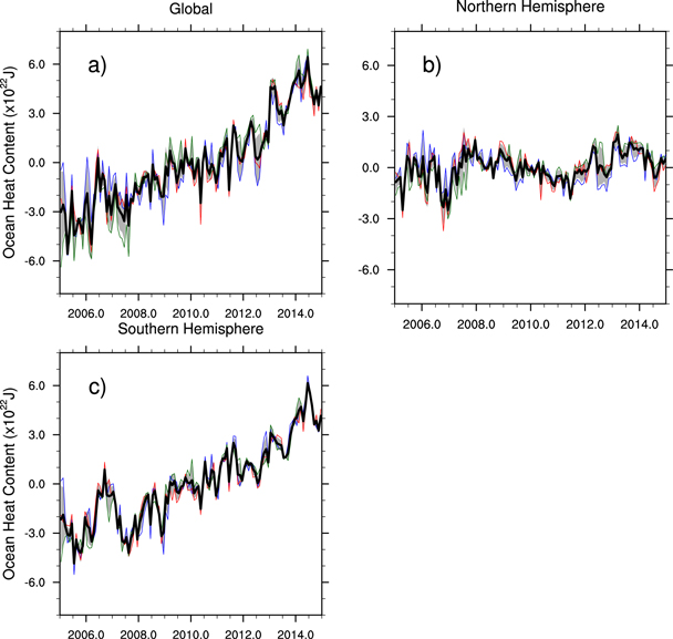
Figure 1. Ocean heat content change above 2000 m depth with respect to the temperature climatology. Curves show estimates based on SCRIPPS (blue curves), IPRC (red curves), JAMSTEC (green curves) and the mean estimate (black curves) for (a) the global ocean (between ± 65° of latitude), (b) the northern hemisphere and (c) the southern hemisphere. The grey envelope denotes one standard deviation around the mean.
Download figure:
Standard image High-resolution imageTable 1. Ocean heat content trends estimated over 2005–2014 and 2006–2013 for SCRIPPS, IPRC, JAMSTEC gridded products and the mean estimate. Bold numbers represent the equivalent heating rates in W.m−2 (Values are normalized by the ocean surface of 350 × 1012 m2). Error uncertainties denote formal errors from linear fit at 1-sigma for the individual Argo gridded products. For the mean estimates we perform a weighted least squares fit to the monthly observations where the weights are chosen to equal the reciprocal variance of the three Argo gridded fields to estimate errors at 1-sigma.
| Trends over 2005–2014 (x1021 J yr−1) and heating rates (W m−2) | Global ocean (65°S–65°N) | Southern hemisphere (65°S-0°N) | Northern hemisphere (0°S-65°N) | Trends over 2006–2013 for the global ocean (as in Roemmich et al 2015) |
|---|---|---|---|---|
| SCRIPPS | 7.19 ± 0.5 | 7.34 ± 0.43 | −0.15 ± 0.28 | 6.07 ± 0.61 |
| 0.65 ± 0.05 | 0.66 ± 0.04 | −0.01 ± 0.02 | 0.55 ± 0.05 | |
| IPRC | 7.87 ± 0.45 | 7.04 ± 0.40 | 0.83 ± 0.35 | 7.4 ± 0.6 |
| 0.71 ± 0.04 | 0.63 ± 0.04 | 0.07 ± 0.03 | 0.67 ± 0.05 | |
| JAMSTEC | 10.18 ± 0.38 | 7.93 ± 0.33 | 2.24 ± 0.27 | 9.62 ± 0.55 |
| 0.92 ± 0.04 | 0.71 ± 0.03 | 0.20 ± 0.03 | 0.87 ± 0.05 | |
| Mean estimate | 8.41 ± 1.56 | 7.44 ± 3.31 | 0.97 ± 3.28 | 7.69 ± 1.54 |
| 0.76 ± 0.14 | 0.67 ± 0.30 | 0.09 ± 0.30 | 0.69 ± 0.14 |
We have partitioned the OHC around the equator to quantify the respective contribution of each hemisphere. Figures 1(b) and (c) show the hemispheric contributions (north and south, respectively) to the global OHC for the upper 2000 m depth from the equator to 65° of latitude. Over 2005–2014, the southern hemisphere appears to explain a large part of the linear increase of the global OHC change (figure 1(c)) with a linear trend of 7.44 ± 3.31 × 10²¹ J yr−1 (based on the mean estimate between the three Argo products) ranging from 7.04 ± 0.40 × 10²¹ (IPRC) to 7.93 ± 0.33 × 10²¹ J yr−1 (JAMSTEC) very similar to the global estimate (cf table 1) whereas the northern hemisphere explains 0.97 ± 3.28 × 10²¹ J yr−1 ranging from −0.15 ± 0.28 × 10²¹ (SCRIPPS) to 2.24 ± 0.27 × 10²¹ J yr−1 (JAMSTEC). In terms of heating rates and over 2005–2014, the mean values are 0.67 ± 0.30 and 0.09 ± 0.30 for the southern and northern hemisphere, respectively (per unit of the ocean surface of 350 ×1012 m2).
In other words, the southern hemisphere explains about 90% of the net ocean heat uptake for the past decade over 2005–2014 and 10% is due to the northern hemisphere (based on the mean time series). It is worth noting that both hemispheres exhibit substantial interannual variability around the trend (figures 1(b), (c)). Overall, we note a good agreement between the three groups.
The ocean heat uptake asymmetry previously described between the two hemispheres is striking and motivate us to investigate the specific regions and depths of such detected warming differences. Thus, figure 2(a) presents the globally averaged depth-dependent temperature trends, over 2005–2014, as a function of depth. As in figure 1, the blue, red and green curves represent OHC estimates from SCRIPPS, IPRC and JAMSTEC while the black curve denotes the mean estimate from the latter. The temperature increase ranges from about 0.008 °C yr−1 to 0.014 °C yr−1 above 300 m depth (values from the mean estimate) over 2005–2014. Below 300 m depth, we find a global ocean warming throughout the water column. Therefore, we found a slight temperature increase with a second maximum near 900 m depth of about 0.004 °C yr−1 (values from the mean estimate). It is important to note the large impact of such temperature change (even if it is a small amount compare to the upper layers) because of the huge mass of seawater down to 2000 m depth that can store a large amount of heat. The overall agreement between the datasets supports a robust ocean warming for the last decade between 2005 and 2014. However, we note a larger spread around the mean for the groups above 900 m depth associated with warmer trends for JAMSTEC product than for SCRIPPS or IPRC gridded fields. Below 900 m depth, we note a better agreement with a smaller spread around the mean estimate.
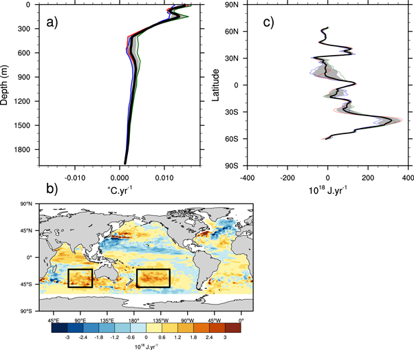
Figure 2. (a) Depth dependent temperature trends versus depth for the SCRIPPS (blue curve), IPRC (red curve), JAMSTEC (green curve) and the mean estimate (black curve). (b) Ocean heat content trend map, 0–2000 m, from the SCRIPPS data (1018 J yr−1). (c) Zonally integrated ocean heat content (1018 J yr−1) for the SCRIPPS (blue curve), IPRC (red curve), JAMSTEC (green curve) and the mean estimate (black curve). The grey envelope denotes one standard deviation around the mean.
Download figure:
Standard image High-resolution imageFigure 2(b) shows the spatial distribution of OHC trends (based on SCRIPPS data only, 1018 J yr−1). We only present the SCRIPPS product because it is representative of all products. The trend map reveals large warming structures centered to the north and the south-east Indian ocean and the south Pacific ocean. We also find a warming structure located in the south Atlantic ocean but with less amplitude than the previous identified regions. Interestingly, we highlight compensations between warming and cooling structures for the north Pacific and north Atlantic oceans with north-south and west-east structures, respectively. Note that the warming patterns for the Pacific and Atlantic oceans coincide with the Kuroshio and Gulfstream currents suggesting a strong role of ocean circulation to the heat redistribution. Furthermore, the north-south pattern observed in the north Pacific ocean might be a consequence of the decadal variability of the Kuroshio extension (Taguchi et al 2007). Our results confirm the recent findings on upper ocean heat content variations described by Roemmich et al (2015) over 2006–2013 and by Wijfells et al (2016) over 2006–2014. It is worth noting the good agreement with the observed and thermosteric sea level trend maps (Llovel and Lee 2015) compared to OHC trend map confirming the importance of temperature changes to regional sea level trends (Cazenave and Llovel 2010, Stammer et al 2013).
Figure 2(c) depicts the zonally integrated OHC change (1018 J yr−1) for all groups. We clearly identify the hemispheric asymmetry of warming around the equator as already mentioned (see figures 1(a), (b) and (c)). We find two maxima of warming for the 2 hemispheres around 40° of latitude with higher amplitudes for the southern hemisphere. Nevertheless, we find some discrepancies between the Argo products around 10°N–30°N. These differences can explain the spread in the trend estimates previously reported for the global OHC time series and trend estimates (see table 1). Otherwise, the Argo products agree on the southern ocean warming and they all converge towards a maximum warming around 40°S corresponding to the center of the subtropical gyres with a large contribution from the south-east Indian and south Pacific oceans (as previously reported in Roemmich et al 2015 and Wijfells et al 2016). Why the south Indian and Pacific oceans experience such a recent upper ocean warming? What are the physical processes involved in such a rapid warming? To answer these questions, we now investigate the role of surface atmospheric flux in generating such a warming pattern.
For that purpose, we first analyze the OHC time series over those regions (represented by the black boxes in figure 2(b)). Figure 3(a) shows the ocean heat content change (down to 2000 m depth) for the south Pacific ocean (figure 3(a)) and for the south-east Indian ocean (figure 3(b)) computed over two boxes centered to the maximum of warming over 185°E–240°E/20°S–50°S and 70°E–110°E/20°S–50°S, respectively (note that the colors are the same as in figure 1). The three Argo-based gridded products agree on an OHC increase for the recent decade. The south Pacific ocean appears to explain a significant part of the linear increase of the global OHC change (cf figure 1(a)) with a mean linear trend of 1.96 ± 1.09 × 10²¹ J yr−1 for 2005–2014 ranging from 1.75 ± 0.08 × 10²¹ (SCRIPPS) to 2.16 ± 0.11 × 10²¹ J yr−1 (IPRC) that corresponds to 23% of the net global ocean warming. This warming ranges between 0.15 ± 0.008 W.m−2 (SCRIPPS) to 0.19 ± 0.01 W m−2 (IPRC) with a mean estimate of 0.18 ± 0.1 W m−2 in terms of equivalent heating rate (per unit of the ocean surface of 350.1012 m2) over 2005–2014. The south-east Indian ocean displays an ocean heat content increase of 1.44 ± 1.12 J yr−1 ranging from 1.26 ± 0.1 J yr−1 (SCRIPPS) to 1.55 ± 0.13 J yr−1 (IPRC). In terms of heating rate, the upper ocean warming ranges between 0.11 ± 0.01 W m−2 (SCRIPPS) to 0.14 ± 0.015 W m−2 (IPRC) with a mean value of 0.13 ± 0.1 W m−2 that corresponds to 17% of the net ocean heat uptake for 2005–2014 (per unit of the ocean surface being 350 × 1012 m2). The south Pacific ocean presents a quite linear increase from 2005 to 2010 and then, an abrupt large OHC increase in 2011 following with large interannual variability afterwards. For the south-east Indian ocean, we find a linear increase from 2005 to 2010 and then large interannual variability. The two considered regions display an OHC increase for the beginning of the period following by interannual variability and a slowdown in the linear increase. This is suggestive of changes in ocean heat content due to possible change in local surface heat fluxes and changes in ocean heat content due to ocean dynamics (e.g., Ekman pumping, advection, diffusion, wave propagation or eddies).
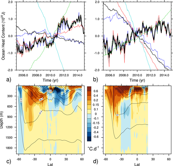
Figure 3. Ocean heat content change above 2000 m depth with respect to the temperature climatology for (a) the south Pacific ocean between 185°E–240°E and 20°S–50°S and for (b) the south-east Indian ocean 70°E–110°E and 20°S–50°S (Solid curves show estimates based on Argo gridded products from SCRIPPS -blue curves-, IPRC -red curves-, JAMSTEC -green curves- and the mean estimate -black curves-; dashed curves show estimates from net surface heat flux anomalies from ERA-interim –blue curves-, NCEP –red curves-, MERRA –light green curves-, JRA—cyan curves- and the mean estimate—black curve-). Zonally-averaged temperature trends (°C yr−1, latitude versus depth, the black lines represent the isopycnal surfaces) from the SCRIPPS data over 2005–2014 for (c) the south Pacific ocean between 185°E–240°E and 20°S–50°S and for (d) the south-east Indian ocean 70°E–110°E and 20°S–50°S.
Download figure:
Standard image High-resolution imageTo further investigate this large regional warming, we have computed the zonally-averaged temperature anomaly trends (based on SCRIPPS data only) computed between 185°E–240°E and 60°S–60°N (figure 3(c)) and between 70°E–110°E and 60°S–20°N (figure 3(d)). The black lines represent the mean isopycnal surfaces computed over 2005–2014. We find large warming structures extending to 2000 m for both the south Pacific and south-east Indian oceans with the maximum warming structures above 600 m depth between 30°S–50°S associated with values ranging from 0.1 °C dec−1 to 0.6 °C dec−1 over 2005–2014. For the Pacific regions, we clearly identify the different behavior between the two hemispheres. Interestingly and in each case, the warming trends follow the isopycnal surfaces suggesting a possible heat penetration into deeper layers from 50°S to the equator. This is also suggestive of a possible contribution from surface atmospheric forcing. Because of the strong evidence of surface atmospheric changes, we analyze the different surface atmospheric flux contribution to the conspicuous upper ocean warming in the following section.
3.2. Surface forcing contribution
In this section, we investigate the contribution of surface forcing to the south Pacific and south-east Indian upper ocean warming patterns. Temperature changes can be due to changes in local surface heat forcing, local Ekman pumping and contribution from ocean dynamics due to remote forcing and intrinsic ocean variability. To examine these factors, we examine the local surface heat flux and the wind stress curl change that induces Ekman pumping.
We first investigate the contribution of the local surface heat flux over the south Pacific and the south-east Indian oceans. The dashed curves of figures 3(a) and (b) represent the implied OHC change due to the net surface heat flux change from ERA-interim (blue), NCEP (red), MERRA (green) and JRA (cyan) atmospheric reanalysis and the mean estimate (back curves). Clearly, the individual implied OHC change display very different behavior for the two considered regions over 2005–2014. For the south Pacific ocean, the different implied OHC trends depict large spread and estimates amount of −0.55 × 10²¹ J yr−1 (ERA-Interim), 1.24 × 10²¹ J yr−1 (NCEP), 6.42 × 10²¹ J yr−1 (MERRA) and −10.5 × 10²¹ J yr−1 (JRA). We find a linear trend of −0.85 ± 6.14 × 10²¹ J yr−1 for the mean estimate computed over 2005–2014. For the south-east Indian ocean, the implied OHC trends account for −3.41 × 10²¹ J yr−1 (ERA-Interim), 6.20 × 10²¹ J yr−1 (NCEP), 2.48 × 10²¹ J yr−1 (MERRA) and −10.12 × 10²¹ J yr−1 (JRA) with a linear trend of –4.31 ± 4.59 × 10²¹ J yr−1 for the mean estimate over 2005–2014. The two mean estimates are not statistically different from zero depicting the large spread from the four atmospheric reanalysis. These results highlight the imbalance in the climatological estimates for the atmospheric reanalysis, especially for MERRA and JRA solutions. Even though the annual cycle is quite well resolved for the atmospheric reanalysis (not shown), the different models differ in the time mean estimates. It is not surprising that the analysis of surface net heat flux is not conclusive because of the remaining errors of surface heat flux fields from the atmospheric reanalysis (Dee et al 2011). However, the discrepancies between the OHC changes due to the local net heat flux and identified Argo products highlight the possible contribution of oceanic processes (such as advection and diffusion components). This result motives us to investigate the wind-driven contribution to the OHC change identified by Argo floats.
Thus, we investigate the change in wind stress curl over 2005–2014. Figures 4(a) and (b) presents the meridional mean wind stress curl for 2005–2007 (dashed curves) and 2012–2014 (solid curves) from ERA-Interim (blue curves), NCEP (red curves), MERRA (green curves), JRA-55 (cyan curves) and the mean estimate (black curves) for the south Pacific and south-east Indian oceans, respectively. We have chosen these two periods to investigate the wind stress curl because of the different behavior of the upper ocean heat content change for the two considered regions (as previously discussed in figures 3(a) and (b)) over 2005–2014. All atmospheric reanalysis agree on a poleward displacement of the meridional mean wind stress curl of about 2° of latitude based on the mean estimate (black curves) for the south Pacific ocean. For the south-east Indian ocean, the poleward shift of mean wind stress curl is smaller than for the Pacific region. Therefore, in both cases, the zero-curl line has shifted to the south. This shift of wind stress curl produces a change in Ekman transport because of the change in Ekman convergence. According to our analysis, the maximum of mean wind stress curl is around 36°S–38°S for the Indian ocean and 44°S–46°S for the south Pacific ocean.
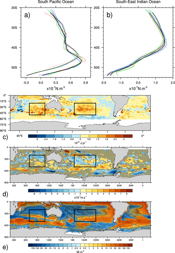
Figure 4. Meridional-averaged wind stress curl (x10−7 N m−3) from ERA-Interim (blue curves), NCEP (red curves), MERRA (green curves), JRA-55 (cyan curves) and the mean estimates (black curves) over 2012–2014 (solid lines) and 2005–2007 (dashed lines) for (a) the south Pacific ocean between 185°E–240°E and for (b) the south-east Indian ocean between 70°E–110°E. (c) same as figure 2(b) for the southern hemisphere, (d) Map of mean Ekman pumping differences between 2012–2014 and 2005–2007 periods (×10−7 m.s−1). (e) Mean net surface heat flux (W m−2) over 2005–2014. The Ekman pumping differences and the mean net heat flux represent the mean between ERA-Interim, NCEP, MERRA and JRA-55. The stippled regions denote values not different from zero at one standard deviation.
Download figure:
Standard image High-resolution imageTo confirm this Ekman pumping intensification, we have computed the mean Ekman pumping difference between 2012–2014 minus 2005–2007 for all the atmospheric reanalysis considered in this study. Figure 4(d) depicts the Ekman pumping mean differences. The stippled regions denote mean estimate not statistically different from zero at one standard deviation. Based on figure 4(d), we clearly identify an increase of Ekman pumping between 44°S and 60°S for the south Pacific ocean and between 40°S and 58°S for the south-east Indian ocean consistent among the different atmospheric reanalysis over 2005–2014. This Ekman pumping deepens the isopycnal surfaces that can enhance heat penetration into the deeper layer of the ocean (as previously suggested while discussing figures 3(c) and (d)). However, such a mechanism is not adiabatic and involves heat input to the ocean.
Then, figure 4(e) shows the mean surface heat flux based on the 4 atmospheric reanalysis. The stippled points represent values not significantly different from zero at one standard deviation. Positive values denote a heat gain by the ocean. Over the subtropical south-east Indian (70°E–110°E and 20°S–50°S) and south Pacific oceans (185°E–240°E and 20°S–50°S), we find a negative contribution of mean surface heat flux being −10.02 W m−2 and −1.68 W m−2, respectively, over 2005–2014 that cannot explain the observed upper ocean warming identify by the different Argo gridded products (as already discussed in figures 3(a) and (b)). However, we find positive net heat surface flux between 40°S and 50°S for the southern Pacific and south of 45°S for the Indian ocean. The latitude band with the largest surface heat flux change does not coincide with the maximum ocean warming spatial pattern. The latter pattern is spatially correlated with the change in Ekman pumping reflecting the role of Ekman transport. The southern shift of wind stress curl enhances a northward Ekman transport. Supposing the Ekman layer does not exceed 100-meter depth in those regions, the mean integrated Ekman transport can be assessed with the surface wind stress. Therefore, we can easily estimate the zonally integrated meridional temperature transport (Stammer et al 2003) by combining the Ekman transport with the OHC inferred by Argo products. We find an increase of 5.87 ± 0.26 × 10²² J and 1.86 ± 1.02 × 10²² J in the mean Ekman transport convergence where the Ekman pumping is maximum between 2005–2007 and 2012–2014 for the south Pacific (44°S–60°S) and south-east Indian (50°S–58°S) oceans, respectively. Estimates are computed using the SCRIPPS data along with the four atmospheric reanalysis considered in the study to assess the consistency of the results. Our results suggest an increase of heat content change due to an increase of Ekman transport convergence for the south Pacific and south-east Indian oceans instead of a local contribution of net heat surface flux.
3.3. Ocean heating rates and net TOA flux
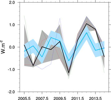
At global scale, the net TOA flux and the ocean heating rates should be in phase with each other (Loeb et al 2012) because the oceans have stored about 90% of the Earth's energy imbalance over 1970–2010 (Rhein et al 2013, Palmer and McNeall 2014). Figure 5 shows the interannual variability of annual global averaged of the net TOA flux from CERES (cyan curve). The blue envelope denotes the uncertainty of 0.31 W m−2 in CERES net TOA flux for each year that is more appropriate for investigating the year-to-year variations as suggested by recent studies (Loeb et al 2012, Trenberth et al 2014). The CERES satellite data do not exhibit the absolute measure of the TOA energy flux because of instrument limitations. Therefore, the EBAF product is anchored to an estimate of ocean heat content change (Loeb et al 2012). As we are focusing our analysis on interannual variability, we have removed the mean estimate from all curves plotted in figure 5. We also compare net TOA time series with annual heating rates from the Argo products (per units of the Earth's surface being 510 × 1012 m2) computed above 2000 m depth. We find significant interannual variability of ocean heating rates ranging from −1 to 1 W m−2 larger than the net TOA flux deduced by CERES data but comparable within uncertainties. We find a correlation coefficient of 0.53 between the mean ocean heating rate based on Argo products and the net TOA flux from CERES measurements. However, we highlight large spread between the ocean heating rates based on the different datasets and disagreement compared with the net TOA flux (before 2010). These differences might be due to unsampled regions from Argo floats (such as marginal seas, continental shelf and high-latitude regions and/or deep ocean below 2000 m, von Schuckmann et al 2016), a significant contribution from another climate reservoir and undetected errors from the observing systems. It is worth noting the importance of quality control tests made on the raw Argo data -as previously discussed in the data and method section- to best assess the consistency between the net TOA Earth energy budget and the ocean heating rates.
Figure 5. Comparison between the net top-of-the-atmosphere flux and the ocean heating rates at annual basis with respect to their time mean (normalized by the Earth's surface of 510 × 1012 m2). The cyan curves represents the net TOA flux from CERES. The blue envelope denotes CERES flux uncertainties of 0.31 W m−2 as suggested by Loeb et al (2012). The ocean heating rates from SCRIPPS (blue), IPRC (red), JAMSTEC (green) and the mean estimate (black) are overlaid. The grey envelope denotes one standard deviation around the mean of the ocean heating rates.
Download figure:
Standard image High-resolution image
The net TOA flux budget shows significant interannual variability that seems to be linked to natural variability. For instance, the El Niño-Southern Oscillation events affect the Earth's energy budget through changes in energy flux exchange between the ocean tropical Pacific ocean and the atmosphere. During the La Niña conditions, the central and eastern tropical Pacific ocean experience cold sea waters creating high atmospheric pressure and clear skies favoring the incoming short wave radiation (Trenberth et al 2002, Trenberth and Fasullo 2012). The excess heat is redistributed by ocean circulation and builds up in the tropical western Pacific ocean feeding the Warm Pool until the next El-Niño event spreads the warm water across the Pacific. During an El-Niño event, the surface warm water along with the wind enhances evaporation that cools the ocean, moistening the atmosphere and creates large atmospheric convection associated with large clouds limiting the incoming short wave radiations (Trenberth and Fasullo 2012). Therefore, the ENSO variability may contribute to the interannual variability of the Earth's energy budget.
4. Discussion and conclusions
Quantifying the OHC is essential for understanding the response of the climate system to radiative forcing because the oceans are the dominant reservoir of heat on Earth. In this study, we have investigated the OHC change inferred by Argo gridded products provided by three different research groups. In overall, we show the good agreement between the different products (correlation coefficients higher than 0.85). We find a decadal increase of OHC of 8.41 ± 1.56 × 10²¹ J yr−1 (mean estimate ranging from 7.19 ± 0.5 × 10²¹ to 10.18 ± 0.38 × 10²¹ J yr−1 depending on hydrographic analysis used) corresponding to an equivalent heating rate of 0.76 ± 0.14 W m−2 (per unit of the ocean surface being 350 ×1012 m2) over 2005–2014. Note that the Argo coverage is not perfect (see white areas in figure 2(b) for instance) and coastal regions, marginal seas and semi-enclosed seas are not well sampled by the floats (Abraham et al 2013) along with high latitude regions. We assume that the sensitivity of Argo-based OHC changes to unsampled regions is small. A recent study has reached the same conclusion in analyzing the global average sea surface temperature from different products (Roemmich et al 2015). Our decadal estimate compares well with the value from the last IPCC-AR5 report of 0.71 W m−2 for 1993–2010 (Rhein et al 2013). As satellite measurements of the net TOA flux are more accurate for interannual variability than for the absolute value (determined as the difference between the incoming and outgoing radiation), a precise quantification of global OHC appears important to constrain the Earth's energy budget. However, as already mentioned, some regions are not well sampled by Argo floats and efforts are undertaken to extend Argo's network to global coverage. This would help to reduce uncertainties related to ocean heat uptake estimations.
One goal of this study is to localize the regions with the largest heat uptake for the recent decade. Therefore, we show that the southern and the northern hemispheres explain about 90% and 10% of the net global OHC increase, respectively. Even if some discrepancies have been found in our analysis among the considered hydrographic products, we found a reasonably good agreement among them. Furthermore, we find that the warming is centered at 40°S which corresponds to the center of the subtropical gyres with two main structures located at the Indian and Pacific oceans. We find a poleward shift of the mean wind stress curl for the south Pacific ocean and for the south-east Indian ocean, based on four atmospheric reanalysis, that could explain the upper ocean warming identified in the south Pacific and south-east Indian oceans instead of local net surface heat flux contribution. This poleward shift suggests a change in Ekman transport associated with a change in Ekman convergence. We find and increase of Ekman mean transport convergence of 5.87 ± 0.26 × 10²² J and 1.86 ± 1.02 × 10²² J for the south Pacific and the south-east Indian oceans, respectively. However, these estimates are larger than the OHC increase especially for the south Pacific ocean to explain the entire OHC increase observed by Argo floats. Other mechanisms not considered in the study may contribute to the observed OHC increase for the two considered regions. Previous studies discussed the physical processes responsible for ocean heat uptake south of 50°S to the midlatitude (Johnson and Orsi 1997, Wong et al 1999) based on hydrographic data. Isopycnal surfaces appear to be steep as seen in figures 3(c) and (d) and sink into deeper layers. Surface Ekman transport, enhanced by poleward-intensifying wind carries water northward gaining heat from the atmosphere before sinking along the isopycnals within the Antarctic Intermediate Water or Mode Water. Therefore, the heat penetrates into the ocean following the isopycnal surfaces and tends to warm the midlatitude band at depth. However, such a mechanism requires an increase of heat input from the atmosphere. We find a possible positive contribution of mean surface heat flux from atmospheric reanalysis south of 50°S for the Pacific and Indian oceans. However, the mean surface heat flux value does not entirely explain the subsurface warming of the midlatitude band revealed by Argo floats probably due to physical processes not considered in our analysis or due to the remaining errors associated with the heat flux estimates inferred by atmospheric reanalysis. We have to keep in mind that one fundamental limitation with the atmospheric reanalysis is the accuracy of the data. The ability to simulate real surface fluxes lies in the quality and availability of observations that are quite sparse over the oceans (Dee et al 2011).
Therefore, one limitation of our study is the complete description of the different mechanisms involved in the observed warming identified by the different Argo products. Further analyses are required to better ascertain the mechanisms involved behind the heat penetration into the two identified regions. Taking advantage of an ocean general circulation model that can reproduce the observed upper ocean warming would be helpful to establish the respective contribution of ocean dynamics and circulation to the observed upper ocean warming over the last decade. Over a longer time period and using coupled climate models, Cai et al (2010) investigated the mechanisms involved in the fast warming rate of the southern midlatitude between the 1950s and the 2000s. The authors highlight the importance of poleward-strengthening winds along with poleward shift of the southern hemisphere gyres and the Antarctic Circumpolar Current to account for the fast ocean warming instead of local heat surface flux changes. Because their study focuses on interdecadal time scales, more work is needed to fully understand the causes and mechanisms involved in the identified ocean warming for the past decade highlighted in this study.
We also investigate the annually averaged ocean heating rates with the net TOA flux inferred by CERES. We find large interannual variability of the net TOA flux in good agreement with ocean heating rates. Thus, we confirm that the yearly mean ocean heating rate is comparable to the net TOA flux for the last decade (Loeb et al 2012) within the uncertainties. However, we find some disagreements before 2010 that could be due to unsampled regions and/or the significant contribution to another climate reservoir and/or larger errors from the different datasets. We conclude that the ocean (above 2000 m depth) contributes significantly to the net TOA flux at interannual time scales as suggested in recent literature (Loeb et al 2012, Rhein et al 2013). Furthermore, we also suggest that there is currently no strong evidence of 'missing energy' in the climate system as it has recently been speculated (Trenberth and Fasullo 2010) due to remaining large uncertainties. Ongoing development of new Argo floats going down to 4000 m/6000 m depth and efforts to extend Argo's network to global coverage will reduce uncertainties and provide accurate data to investigate the ocean contribution to the Earth's energy budget and the future sea level rise (Johnson and Lyman 2014, Johnson et al 2015).
Acknowledgments
William Llovel is supported by a CNES post-doctoral fellowship and carried out at CERFACS. The Argo data were collected and made freely available by the International Argo Program and the national programs that contribute to it (http://argo.ucsd.edu and http://argo.jcommops.org). The Argo Program is part of the Global Ocean Observing System.