

Abstract
Actual land evapotranspiration (ET) is a key component of the global hydrological cycle and an essential variable determining the evolution of hydrological extreme events under different climate change scenarios. However, recently available ET products show persistent uncertainties that are impeding a precise attribution of human-induced climate change. Here, we aim at comparing a range of independent global monthly land ET estimates with historical model simulations from the global water, agriculture, and biomes sectors participating in the second phase of the Inter-Sectoral Impact Model Intercomparison Project (ISIMIP2a). Among the independent estimates, we use the EartH2Observe Tier-1 dataset (E2O), two commonly used reanalyses, a pre-compiled ensemble product (LandFlux-EVAL), and an updated collection of recently published datasets that algorithmically derive ET from observations or observations-based estimates (diagnostic datasets). A cluster analysis is applied in order to identify spatio-temporal differences among all datasets and to thus identify factors that dominate overall uncertainties. The clustering is controlled by several factors including the model choice, the meteorological forcing used to drive the assessed models, the data category (models participating in the different sectors of ISIMIP2a, E2O models, diagnostic estimates, reanalysis-based estimates or composite products), the ET scheme, and the number of soil layers in the models. By using these factors to explain spatial and spatio-temporal variabilities in ET, we find that the model choice mostly dominates (24%–40% of variance explained), except for spatio-temporal patterns of total ET, where the forcing explains the largest fraction of the variance (29%). The most dominant clusters of datasets are further compared with individual diagnostic and reanalysis-based estimates to assess their representation of selected heat waves and droughts in the Great Plains, Central Europe and western Russia. Although most of the ET estimates capture these extreme events, the generally large spread among the entire ensemble indicates substantial uncertainties.
Export citation and abstract BibTeX RIS

Original content from this work may be used under the terms of the Creative Commons Attribution 3.0 licence.
Any further distribution of this work must maintain attribution to the author(s) and the title of the work, journal citation and DOI.
1. Introduction
Climate impact models are frequently used to quantify and analyse the effects of environmental changes in various socio-economic and environmental sectors under a given scenario design. However, the interpretative power of individual impact model simulations is severely limited due to the lack of thorough estimates of the full range of inter-model and inter-sectoral uncertainties Frieler et al (2015). The second phase of the Inter-Sectoral Impact Model Intercomparison Project (ISIMIP2a) provides a new framework deemed to gain better uncertainty estimates to model-based projections through an integrative approach Warszawski et al (2014). For the critical assessment of extreme events, it is absolutely necessary to be aware of these uncertainties, concerning both the spread among the ISIMIP simulations as well as biases of the multi-model mean with respect to independent observation-based estimates from the recent past.
Key impact variables such as irrigation water demand or agricultural productivity are physically controlled by the partitioning of energy at the land surface, which largely depends on total evapotranspiration (ET, e.g. Betts et al 1996). As ET accounts for more than half of the precipitation fluxes in many regions, it is an important parameter controlling hydrological extreme events, in particular when considering its potential to amplify droughts and heat waves through coupling with soil moisture (e.g. Seneviratne et al 2010). However, to analyse such extreme events in greater detail, it is absolutely necessary to be aware of the full range of uncertainties inherent in different estimates of ET. In an early but comprehensive comparison of various land surface models within the Project for Intercomparison of Land-surface Parameterization Schemes (PILPS, Henderson-Sellers et al 1993, Henderson-Sellers et al 1996), enormous uncertainties in the representation of evaporation among different land surface schemes have been found (Shao and Henderson-Sellers 1996, Chen et al 1997, Wood et al 1998, Pitman et al 1999). Although considerable progress has been made since Pitman (2003), land evaporation remains to be one of the most uncertain components of the global hydrological cycle to date (e.g. Fisher et al 2017). It is hence not surprising that a recent ensemble product of global ET estimates still reveals substantial uncertainties, which are comparable to the magnitude of uncertainties in precipitation estimates Mueller et al (2013). To thoroughly analyse extreme events within the ISIMIP2a framework, it is thus a prerequisite to precisely assess the magnitude of common ensemble statistics (mean, median and interquartile ranges, IQRs) of presently available ET estimates across datasets/models and sectors, and to further attempt to identify potential causes for differences between these estimates.
Uncertainties in estimates of ET can be due to multiple interrelated factors, including (but not limited to) the choice of the model or the forcing, the data category (model-based estimates from a specific sector, diagnostic or reanalysis-based estimates), the number of soil layers in the model and the ET scheme. Studies from the recent past have mainly focussed on the latter issue: the difficulties of choosing the most appropriate ET scheme for specific applications (e.g. Kay et al 2013, Bormann 2011), which can even translate into ambiguities in the interpretation of the evolution of past global drought conditions (Sheffield et al 2012, Seneviratne 2012). Numerous papers confirm that the most widely used FAO56 Penman-Monteith formulation produces the most reasonable estimation of potential evaporation (Ortega-Farias et al 2004, DehghaniSanij et al 2004, Donohue et al 2010, Prudhomme and Williamson 2013), whereas others see similar performance of the Priestley-Taylor (Shaw and Riha 2011, Kingston et al 2009) or the Hargreaves formulation Kingston et al (2009), and a few do not make any clear recommendation (Schulz et al 1998, Kite and Droogers 2000). Other studies even state that Penman-Monteith does not essentially yield the best estimates (Weiß and Menzel 2008, Douglas et al 2009 and Xu and Chen 2005) suggest Priestley-Taylor, Vörösmarty et al (1998) suggest the Hamon method, and (Liu et al 2007, Liu and Yang 2010 and Sperna Weiland et al 2012) recommend the Hargreaves equation, where the latter suggests to use a re-calibrated form of the equation for climate change studies). Given these uncertainties, it is highly appropriate to assess in more detail whether the differences in ET schemes govern the overall differences across available ET estimates, or whether some of the other factors prevail.
Here we make use of the ISIMIP2a framework to assess selected hydrological extreme events by taking uncertainties into account that arise from difficulties in simulating global land ET. The analysis makes use of a large ensemble of ET datasets including models participating in the the global water, biomes and agriculture sectors, and also including other (independent) estimates from the following sources (introduced in more detail in section 2):
- i.An ensemble of diagnostic datasets,
- ii.the EartH2Observe Tier-1 dataset (version 1, Schellekens et al 2017, hereafter referred to as E2O),
- iii.the LandFlux-EVAL initiative (Mueller et al 2013, hereafter abbreviated as LFE), and
- iv.
This variety of datasets allows us to assess the full range of uncertainties captured by simulated or observation-based historical records of ET, and to identify strengths and weaknesses of individual groups of datasets with respect to their potential to reflect regional ET anomalies during extreme events. The ensemble is particularly suitable to draw valuable conclusions on structural differences among the datasets (e.g. to measure the influence of the meteorological forcing dataset employed in each of the model-based estimates).
The remainder of this paper is structured as follows. After a brief introduction to all input datasets in section 2, we present our methodological approach (section 3). This is followed by the presentation and discussion of spatial and spatio-temporal variabilities across the analysed datasets by means of a cluster analysis (section 4.1), after which we examine individual time series of global and regional ET (section 4.2). Section 5 summarizes the main findings of this study.
2. Data
Table 1 lists all datasets used in this study. In total, we assess 11 diagnostic datasets, nine models from E2O, 12 models from the ISIMIP2a agriculture sector, seven models from the ISIMIP2a biomes sector, 11 models from the ISIMIP2a global water sector, two land reanalyses and one composite dataset (the latter consisting of four different realizations). Note that ET estimates from all datasets except from the ISIMIP2a crop model simulations (labelled with asterisks (⁎) in table 1) correspond to estimates of total ET at monthly resolution (hereafter denoted as ETtot). Besides other information, the table also shows the category that each dataset is associated with. In the following, we provide some more information for each of the data categories. Please refer to the publications listed in table 1 for more detailed information on individual datasets.
Table 1. Overview of datasets used in this study sorted by data category and dataset name. ISIMIP2a simulations are printed in bold.
| Meteorological forcing | |||||
|---|---|---|---|---|---|
| dataset | Data category | GSWP3 | PGMFD | WFDEI | Citation |
| FLUXNET-MTE | Diagnostic | Jung et al (2009) | |||
| GETA 2.0 | Diagnostic | Ambrose and Sterling (2014) | |||
| GLEAM V3.1A | Diagnostic | Martens et al (2016) | |||
| MODIS Global ET | Diagnostic | Mu et al (2011) | |||
| PM-MU-LANDFLUX | Diagnostic | Vinukollu et al (2011) | |||
| PML-CSIRO | Diagnostic | Zhang et al (2016) | |||
| PT-FI-LANDFLUX | Diagnostic | Fisher et al (2008) | |||
| SEBS-LANDFLUX | Diagnostic | Su (2001) | |||
| WANG-ET | Diagnostic | Wang et al (2010a, b) | |||
| WB-MTE | Diagnostic | Zeng et al (2014) | |||
| WECANN | Diagnostic | Alemohammad et al (2016) | |||
| HBV-SIMREG | E2O | x | Beck et al (2016) | ||
| HTESSEL | E2O | x | Balsamo et al (2011) | ||
| JULES | E2O | x | Best et al (2011) | ||
| LISFLOOD | E2O | x | Burek et al (2013) | ||
| ORCHIDEE | E2O | x | Krinner et al (2005) | ||
| PCR-GLOBWB | E2O | x | Wada et al (2014) | ||
| SURFEX-TRIP | E2O | x | Oki and Sud (1998) | ||
| W3RA | E2O | x | van Dijk et al (2013) | ||
| WaterGAP3 | E2O | x | Eisner (2016) | ||
| CLM-CROPa | ISIMIP agriculture | x | Drewniak et al (2013) | ||
| EPIC-BOKUa | ISIMIP agriculture | x | x | x | Williams (1995), Izaurralde et al (2006) |
| EPIC-IIASAa | ISIMIP agriculture | x | Balkovič et al (2014) | ||
| EPIC-TAMUa | ISIMIP agriculture | x | Kiniry et al (1995) | ||
| GEPICa | ISIMIP agriculture | x | Liu et al (2007), Folberth et al (2012) | ||
| LPJ-GUESSa | ISIMIP agriculture | x | x | x | Lindeskog et al (2013) |
| LPJmLa | ISIMIP agriculture | x | x | Bondeau et al (2007) | |
| ORCHIDEE-CROPa | ISIMIP agriculture | x | x | Wu et al (2016) | |
| PAPSIMa | ISIMIP agriculture | x | Elliott et al (2014) | ||
| PDSSATa | ISIMIP agriculture | x | Elliott et al (2014) | ||
| PEGASUSa | ISIMIP agriculture | x | Deryng et al (2014) | ||
| PEPICa | ISIMIP agriculture | x | Liu et al (2016) | ||
| CARAIBc | ISIMIP biomes | x | x | x | Dury et al (2011) |
| DLEMc | ISIMIP biomes | x | x | x | Tian et al (2015) |
| JULES-B1 | ISIMIP biomes | x | x | Clark et al (2011) | |
| LPJ-GUESS | ISIMIP biomes | x | x | x | Smith et al (2014) |
| ORCHIDEE | ISIMIP biomes | x | x | x | Krinner et al (2005) |
| VEGASc | ISIMIP biomes | x | x | Zeng et al (2005) | |
| VISIT | ISIMIP biomes | x | x | x | Ito and Inatomi (2012) |
| CLM | ISIMIP global water | x | x | x | Leng et al (2015) |
| DBH | ISIMIP global water | x | x | x | Tang et al (2007) |
| H08 | ISIMIP global water | x | x | x | Hanasaki et al (2008) |
| JULES-W1 | ISIMIP global water | x | x | x | Best et al (2011) |
| LPJmL | ISIMIP global water | x | x | x | Sitch et al (2003) |
| MATSIRO | ISIMIP global water | x | x | x | Pokhrel et al (2015) |
| MPI-HM | ISIMIP global water | x | x | x | Stacke and Hagemann (2012) |
| PCR-GLOBWB | ISIMIP global water | x | x | x | Wada et al (2014) |
| SWBM | ISIMIP global water | x | x | x | Orth and Seneviratne (2015) |
| VIC | ISIMIP global water | x | x | x | Liang et al (1994) |
| WaterGAP2 | ISIMIP global water | x | x | x | Müller Schmied et al (2016) |
| ERA-Interim/Land | Land Reanalyses | Balsamo et al (2015) | |||
| MERRA-2 | Land Reanalyses | Reichle et al (2017) | |||
| LandFlux-EVALb | Compositeb | Mueller et al (2013) | |||
aET estimates from crop model simulations participating in the ISIMIP2a agriculture sector are performed as pure crop runs only reporting growing season ET without the fallow period for a specific crop type and irrigation scenario (see more details in section 2.1). bWe distinguish here between four data subsets: (1) diagnostic datasets only (denoted as LFE DIAGNOSTIC), (2) land surface model (LSM) simulations (LFE LSM), (3) reanalysis datasets (LFE REANALYSES), and (4) all datasets combined (LFE ALL). cAs naturalized runs are not available for these biomes models, we have used varsoc simulations instead (i.e. simulations for which climate, population, gross domestic product, land use, technological progress and other parameters vary over the historical period).
2.1. Model simulations and land reanalyses
We analyse ET from historical simulations of the ISIMIP2a project using all models from the global water, biomes and agriculture sectors that simulate ET using the model's default ET scheme. The simulations used in this analysis are based on three distinct meteorological forcing datasets: the Global Soil Wetness Project Phase 3 (GSWP3, http://hydro.iis.u-tokyo.ac.jp/GSWP3/), the Princeton Global Meteorological Forcing Dataset version 2 (PGMFD v.2, Sheffield et al 2006) and the Water and Global Change (WATCH, Weedon et al 2011) Forcing Data methodology applied to ERA-Interim data (WFDEI, Weedon et al 2014). We use naturalized runs (i.e. without human impact) only, except from a few simulations from biomes models (see table 1). Due to the large number of models involved, we cannot provide a detailed description of each model here, and rather suggest the interested reader to either consider the publications listed in table 1 or to consult the summary information listing the most relevant characteristics of each model (freely accessible via the ISIMIP website, www.isimip.org/impactmodels/).
From the pool of crop model simulations of the ISIMIP2a agriculture sector, we only select harmonized simulations (see Elliott et al 2015 for details). All crop model simulations use fixed fertilizer application rates except for LPJmL and LPJ-GUESS, as fertilizer input is irrelevant for this version of these models. As previously mentioned in table 1, ISIMIP2a crop model simulations are provided as pure crop runs (i.e. assuming a specific crop is growing all over the world), implying that the ET output from these models corresponds to the amount of water evaporated or transpired from a specific crop type under a given irrigation scenario. Among all crop model simulations available within the ISIMIP2a framework, we focus here on ET from non-irrigated maize crops (denoted as ETmaize), as this crop type is among the most dominant crop types in the regions of interest (see section 3.2 and figure A1) and its growing season matches the summertime growing season on the Northern Hemisphere (see figure A2), making the comparison of ETmaize with ETtot more straightforward. Note that additional preprocessing steps are required prior to performing these comparisons (listed in appendix B).
To additionally include simulations used in the scope of other model inter-comparison projects than ISIMIP, we also include estimates from simulations used in the E2O Water Resources Reanalysis v.1 (Schellekens et al 2017). Please refer to the latter publication for a short description of each of the contributing (land surface, global hydrological and simple water balance) models. Note that SWBM is also part of E2O but has been excluded from this ensemble, as its version is identical to the one of SWBM provided in ISIMIP2a. PCR-GLOBWB and Water GAP are also part of both inter-comparison projects, but kept in both ensembles due to differences in the model versions.
Besides the aforementioned simulations, we also analyse ET output from two major land reanalysis products: ERA-Interim/Land and MERRA-2. ERA-Interim/Land has been selected, as it is commonly used as a reference for quantifying land surface conditions (89 citations as of September 14, 2017, according to Web of Science). MERRA-2 is the most recent reanalysis advancement from NASA that uses refined precipitation corrections Reichle et al (2016). Although ET from MERRA-2 is known to have an anomalously high share of bare soil evaporation Schwingshackl et al (2017), the global average of total ET is well within the range of ET from other reanalyses Bosilovich et al (2016), making it a sufficiently good candidate for our analysis.
2.2. Diagnostic estimates
We use an ensemble of recent diagnostic datasets suitable for identifying potential biases in model-based estimates of ET (see table 1). This ensemble consists of some well established ET estimates from the recent past (a subset of those diagnostic datasets has also been used to generate the ensemble of diagnostic ET in LFE, see section 2.3), but also includes more recent datasets such as GLEAM v3.1 Martens et al (2016). Please refer to the references listed in table 1 for further details on the individual datasets. Please note that the version of Fluxnet-MTE employed here uses a modified temperature and precipitation forcing compared to the previous version presented in Jung et al (2009).
2.3. Composite estimates: LandFlux-EVAL
LandFlux-EVAL (LFE) is an ensemble based land ET product that itself is based on individual diagnostic, model and reanalysis products available in the early 2010s Mueller et al (2013), which we use here as a reference dataset (96 citations as of September 14, 2017, according to Web of Science). Although we cannot argue that LFE is free of biases, we can make the conservative assumption that its ensemble statistics (in particular the provided quantile statistics) are a suitable estimate for quantifying the probable range of ET over land. Please note that some of the diagnostic and model datasets used in the LFE ensemble are also included as individual datasets in this analysis, and hence there is some degree of dependency between the diagnostic (model based) estimates and both LFE DIAGNOSTIC (LFE LSM) and LFE ALL.
3. Methods
3.1. Remapping
In order to allow an inter-comparison of all datasets (mostly available at 0.5° resolution), we have bi-linearly interpolated all input data to a 1° × 1° regular latitude-longitude grid (which corresponds to the spatial resolution of LFE). As LFE can be interpreted as an ET reference product (see section 2.3), we favoured to proceed with this lower resolution.
3.2. Study areas
Besides global land (excluding Antarctica), we focus on the following regions (see table 2): (1) the Great Plains region (spatial delineation according to the USGS physiographic divisions of the conterminous US, https://water.usgs.gov/lookup/getspatial?physio), (2) Central Europe (37°N–53°N and 1°W–20°E, representing the European land area with the highest JJA temperature anomalies in summer 2003 according to Schär et al (2004)) and (3) western Russia (50°N–60°N and 35°E–55°E, according to Dole et al (2011)). These regions have been selected, as they contain large areas of agricultural land that has been affected by severe heat waves and droughts during the time period covered by most of the assessed datasets. The spatial extent of the study areas is also indicated in figures A2 and A1. For each of the regions, area averages of ET were derived by weighting each grid cell by its land area (based on ISLSCP II Global Population of the World, Balk et al 2010).
Table 2. List of prominent drought events that have occurred during the study period.
| Region | Drought event year | Citations |
|---|---|---|
| 1987 | Trenberth et al (1988) | |
| Great Plains | 2002 | Pielke et al (2005) |
| 2012 | Hoerling et al (2013) | |
| Central Europe | 2003 | Schär et al (2004) |
| García-Herrera et al (2010) | ||
| Western Russia | 2010 | Barriopedro et al (2011) |
| Hauser et al (2016) |
3.3. Cluster analysis
We apply two distinct approaches to determine the overall level of similarity between the individual datasets focusing on (a) a combination of spatial and temporal variability (replicating the method described and applied in Sanderson and Knutti (2012) and Sanderson et al (2015) for the univariate case) and (b) spatial variability alone (following Mueller et al 2011). For both approaches, we first create a subset only containing data from the period of temporal overlap (1989–2005) using all datasets except from GETA 2.0, MODIS Global ET and WECANN (which are not of sufficient length). If any of the grid cells (from any dataset and time step) contain missing data, values corresponding to those grid cells are removed from all datasets for all time steps. From the m = 75 (m = 89 for ETmaize) datasets remaining, we then proceed as follows:
In approach (a), we first reform the elements of the four-dimensional input field (latitude, longitude, time and dataset) to a two-dimensional matrix X of size m by n (where n corresponds to the number of all non-missing observations) and transform this into anomalies (based on all time steps remaining) ΔX. To only preserve the dominant modes of ensemble variability, a singular value decomposition (SVD) is performed on ΔX and truncated to t = 9 modes (which is well within the range of suitable truncation values found in Sanderson et al (2015)). The corresponding loadings matrix U (size m by t) can now be used to derive the difference matrix Dsvd by calculating pairwise Euclidean distances as
In approach (b), we simply calculate the temporal average (denoted 'tavg') and reform the result to a two-dimensional matrix Y of size m by p (where p corresponds to the number of remaining grid cells, which is the same for all datasets). We then calculate pairwise Euclidean distances δij in between datasets i and j, resulting in the difference matrix Dtavg (dimensioned m by m):
The distance matrices Dsvd and Dtavg are then subjected to hierarchical clustering by applying the hclust function in R statistics software with Ward's clustering criterion (Ward 1963, ward.D2). The results are visualized in R using the Complex Heatmap package (version 1.14.0, available at https://bioconductor.org/packages/release/bioc/html/ComplexHeatmap.html). Clusters arevisually highlighted using a fixed threshold corresponding to the 99th percentile of the distances to enhance comparability of the results. To compare these clusters against the influence of the assessed factors (i.e.the data category, forcing, number of soil layers, ET scheme and model choice) on overall ET variability, we also assess the fraction of variation explained by each of those factors. This is achieved by means of applying a permutational multivariate analysis of variance (PERMANOVA, Anderson 2001) on the Euclidean differences Dsvd and Dtavg.
4. Results and discussion
4.1. Spatio-temporal patterns of global land ET
Figure 1 shows global patterns of time averaged total ET (i.e. excluding crop models) grouped by data category. Spatial patterns of the ensemble averages are mostly similar among data categories and delineate the average location of the governing hydroclimatic regimes, such as the Intertropical Convergence Zone. The ensemble spread (as expressed by the IQR, i.e. the difference between the 75th and 25th percentile) in tropical rainforest regions is generally largest for the ISIMIP simulations and LFE ALL, whereas the uncertainties (in absolute values) in this region are considerably less pronounced in the diagnostic and E2O ensemble. Similarly, the spatial patterns of the relative ensemble spread (shown by means of the quartile coefficient of dispersion, QCD, which is a relative measure of dispersion, Bonett 2006) in the diagnostic ensemble are very well represented by both ISIMIP sectors and by LFE ALL. Although the magnitude of the uncertainties in the diagnostic ensemble is smaller than in the ISIMIP sectors, it is still higher than the relative ensemble spread in E2O. Note, however, that these small inter-model differences are linked to the fact that the E2O models are all forced by WFDEI, while the ISIMIP ensembles consist of three different forcings.
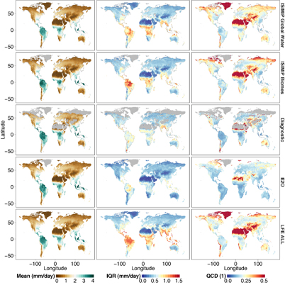
Figure 1. Temporal averages (1989–2005 time period) of monthly ensemble means (left), ensemble IQRs (middle) and ensemble QCDs (right) of ETtot grouped by data category (rows). The diagnostic ensemble is based on all diagnostic datasets except GETA 2.0, MODIS Global ET and WECANN (which have been excluded due to insufficient length). ERA-Interim/Land and MERRA-2 are not shown.
Download figure:
Standard image High-resolution image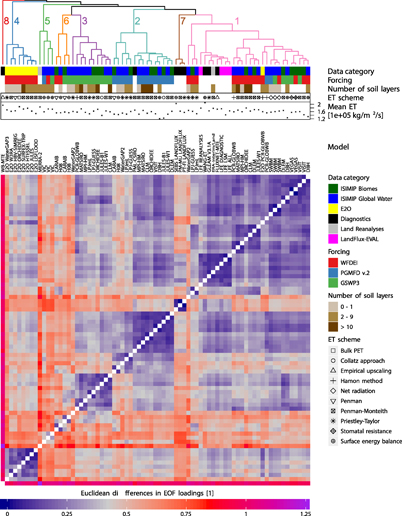
Figure 2. (Previous page) Euclidean differences based on Dsvd (capturing spatio-temporal variabilities) for global land ETtot (coloured matrix). Dataset names are indicated by the column names on top of the matrix (ISIMIP model simulations are printed in bold). For each dataset, the coloured or symbolized rows on top of the matrix indicate the associated data category, the meteorological forcing, the number of soil layers, the ET scheme and the time-average of global land mean ET of each dataset. White boxes or missing symbols indicate that an association is not possible. The dendrogram on the top displays the similarity among the datasets. Colours and numbers indicate clusters (ordered by their size) of datasets with particularly small differences among its members.
Download figure:
Standard image High-resolution image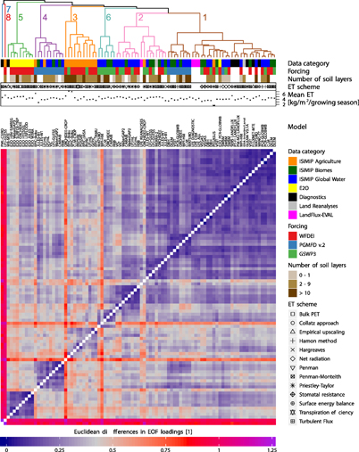
Figure 3. As in figure 2, but for global land ETmaize (note the different units).
Download figure:
Standard image High-resolution imageThe results of the SVD-based cluster analyses are shown in figures 2 (ETtot) and figure 3 (ETmaize). As the associated clusters explain most of the variability among the assessed datasets (i.e. incorporating variability in both their spatialand temporal domains), we treat those as our main results, but occasionally draw comparisons to the clustering results based on time-averaged ET (visualized in figures A3 and figure A4). In the following, we highlight important details of the cluster diagrams by discussing individual parameters potentially having a measurable influence on the differences among the analysed ensemble.
At first glance, we notice a few apparent outliers in the displayed difference matrices, most strikingly for WB-MTE (ETtot), PM-MU CSIRO, MPI-HM and the crop models LPJ-GUESS and ORCHIDEE-CROP (ETmaize only). As the differences among the contributing models are affected not only by the modelling structure but also the calibration process taken, it is not surprising to see such apparent differences between the non-calibrated models LPJ-GUESS and ORCHIDEE-CROP and all other datasets (the less pronounced signal for ORCHIDEE-CROP is potentially due to the fact that this model includes Nitrogen cycling). We also see that the long-term average global land mean ET of these models is not an outlier, suggesting that the differences are mainly due to anomalous patterns in the spatial domain. This is also supported by the clustering results of time-averaged ET, where outliers in the dendrogram mostly coincide with anomalies in the long-term mean (e.g. WANG-ET for ETtot, figure A3 or PEGASUS for ETmaize, figure A4).
The meteorological forcing has, in general, a very noticeable impact on ET estimates when considering variability across both space and time. There are a number of clusters whose members are almost exclusively based on the same forcing (e.g. all PGMFD-forced simulations form a single cluster for ETtot; cluster 2 in figure 2), underlining the dominant role of this parameter. However, the forcing apparently only has very minor influence on the spatial variability of time-averaged ETtot (figure A3), indicating that most of the differences in between the employed forcing datasets are due to differences in the temporal evolution of ET. For ETmaize, there are a few more models for which the forcing dominates the differences, arguably due to a higher sensitivity of these models to diurnal forcings and other parameters which play a more important role when considering crop-specific ET aggregated over growing seasons.
Similarities among the individual datasets can also be reasonably well explained by their data category. While ET simulations from the ISIMIP global water and biomes models are very similar, crop models show substantial differences to all other realizations (the majority of the crop model simulations are members of the same cluster; cluster 3 in figure 3), reflecting the missing (or only rudimentary) representation of crops in the water and biomes models. E2O simulations also share most of their space-time variability (all but one of the E2O simulations fall into the same cluster; cluster 4 in figure 2 and cluster 5 in figure 3). This could be due to stronger similarities among the models participating in this project. Diagnostic datasets mostly show similarities in the spatial variability of the time averages (for ETtot in figure A3, all but two diagnostic datasets are associated with the same cluster). It is also noticeable that ET diagnostics from the LandFlux project (i.e. PM-MU LANDFLUX, PT-FI LANDFLUX and SEBS LANDFLUX) form their own cluster in the spatio-temporal dendrogram (most pronounced in cluster 7, figure 2). For ETtot, we also note that the LFE products are quite similar to most of the diagnostic datasets (sub-tree of cluster 1 in figure 2), adding support that LFE can indeed be used as a reference.
The other two parameters displayed in the cluster diagrams are the (binned) number of soil layers (water and crop models only) and the ET parametrization scheme. These parameters apparently only play a minor role for the clustering. While there are still a couple of instances where the ET scheme seems to contribute to small differences among the datasets (e.g. sub-trees of clusters 1, 2 and 4 in figure 2 indicate that datasets using the Penman-Monteith formulation show particularly little differences), there is no apparent influence of the number of soil layers. It must also be noted that there are many cases where both the ET scheme and the model are the same (e.g. cluster 5 in figure 2), suggesting that (in these cases at least) the associated small differences are due to the identity of the model. These findings are in contrast to what we would have expected from the literature, which suggests that ET schemes may explain a substantial part of the overall variance in ET (see section 1), whereas our results rather suggest that the forcing dominates this variance.
Besides looking at the individual clusters, it is also important to assess the fractional variance in ET for each of the factors considered (figure 4). In all cases, the assessed factors are capable of explaining more than 90% of the variabilities in the distance matrices (Dsvd and Dtavg), and the identified proportions of explained variance are all statistically significant (p < 0.01). Irrespective of the distance metric and the type of ET estimate, differences in the forcing, model choice and ET scheme together account for more than half of the variabilities. In fact, the combined effect of model choice and ET schemes alone can explain at least 48% of the variabilities (which is again in line with previous findings that stress the importance of ET schemes). When considering Dsvd, the forcing plays an important (for ETtot even the leading) role, whereas differences in Dtavg can mainly be explained by the choice of the model. In spite of its minor role for the cluster analysis, the ET scheme can explain more than a quarter of the variabilities.

Figure 4. Fraction of variance in Dsvd (representing spatio-temporal variabilities) and Dtavg (representing spatial variabilities) for both ETtot and ETmaize explained by different factors (coloured shading and numbers [%]). Also shown is the proportion of unexplained variance (grey shading).
Download figure:
Standard image High-resolution image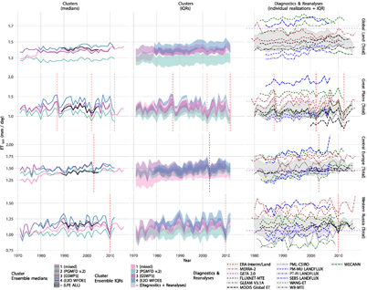
Figure 5. Time series of annual mean ET averaged over global land, the Great Plains, Central Europe and western Russia (rows). The first and second columns show ensemble medians and IQRs of the four largest clusters (numbered 1–4; names in brackets correspond to the dominant meteorological forcing or data category found within each cluster, as displayed in figure 2). Also shown is the median of LFE ALL. The rightmost column shows area averages of individual diagnostic (black, purple, blue and green) and reanalysis datasets (brown), and the associated IQR (grey shading). The long-term average ET estimate from GETA 2.0 is shown as a horizontal purple line. Drought events in the different regions are marked by vertical red lines.
Download figure:
Standard image High-resolution image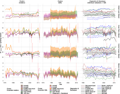
Figure 6. Like figure 5, but for fractional ET for non-irrigated maize crops, also including crop models from the ISIMIP2a agriculture sector. The last year of the global land estimates is excluded here, as it also contains ET from maize crops within the Southern Hemisphere, where the respective growing seasons usually end in the next calendar year (see figure A2).
Download figure:
Standard image High-resolution imageWe now have a good overview of the structural differences among the assessed ensemble of datasets. Based on this information (using the largest sub-ensembles shown in figures 2 and figure 3), we can now go ahead and investigate differences among the clusters with respect to both the temporal evolution of ET and the representation of extreme events.
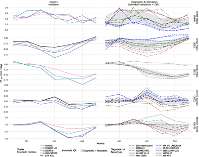
Figure 7. Like figure 5, but for monthly ET anomalies (reference period 1989–2005), excluding GETA 2.0, MODIS Global ET and WECANN. Cluster IQRs are not displayed for clarity. Individual time series are centered at the event years shown in the labels on the right-hand side of each sub-plot.
Download figure:
Standard image High-resolution image4.2. Temporal evolution of global and regional averages of ET
Figures 5 and figure 6 present global and regional time series of both ETtot and ETmaize, respectively. Among the diagnostics- and reanalysis-based estimates we see a few noticeable outliers for both ETtot and ETmaize, most notably SEBS LANDFLUX (for which the global and regional averages exceed the IQR of the entire time span). The magnitude of the spread (IQR) among those estimates is comparable to the magnitude of the spread of the displayed cluster-based sub-ensembles. In the global domain, the diagnostics- and reanalysis-based estimates of ETtot are slightly positively biased with respect to the other sub-ensembles shown. Those differences are most pronounced for cluster 2 (which is also located well below the other cluster ensembles and is also offset with respect to the median of LFE ALL), suggesting an underestimation of global land ETtot, which is potentially related to the dominance of PGMFD-forced model simulations in this cluster. However, the respective sub-ensemble for ETmaize (cluster 4 in figure 6) is well embedded in the overall spread for all regions considered. We also observe that crop models from the ISIMIP agriculture sector tend to disagree more on ETmaize than datasets from the other clusters, although their median is well in agreement with the medians of the other sub-ensembles (cluster 3 in figure 6; note that this ensemble consists of only one model prior to 1979). Except from this, the medians of the clusters agree reasonably well, both in terms of their absolute magnitude (which is close to the median of LFE ALL) and their temporal variability.
The prominent jump in ETtot from 1978–1979 apparent for cluster 1 within the Central European and global domains (figure 5) is due to the switch in the forcing data from WATCH to WFDEI at this time (when considering a sub-ensemble of only WFDEI-forced simulations, this discontinuity becomes even more pronounced, not shown). This artificial change signal is caused by differences in the reanalysis product used to create these datasets (ERA-40 for WFD, ERA-Interim for WFDEI), and is mainly due to the revision in the average aerosol loadings in North Africa and Europe affecting the short-wave incoming solar radiation in these regions (Weedon et al 2014).
A particularly important aspect to assess in greater detail is the response of the different datasets and sub-ensembles to drought events in the study areas (drought years indicated in rows 2–4 in figures 5 and figure 6; in addition, monthly time series for each event year are shown in figure 7). Irrespective of the region and event considered, month-to-month changes in ET anomalies in the displayed sub-ensembles are similar to the changes in the ensemble mean of the diagnostic estimates. However, we note that there is a tendency of the model-dominated sub-ensembles to exaggerate negative ET anomalies (relative to the diagnostic estimates), which could be related to overly strong soil water depletion in some of the model simulations, to models overestimating stomatal closure, to some models not representing irrigation, or to missing non-stomatal flux components.
For each of the considered regions, there has been at least one pronounced drought during the analysed time span (see table 2). While the 1987 Great Plains drought has no apparent influence on ET rates, the events in 2002 and 2012 are characterized by negative ET anomalies apparent in both the displayed clusters and in most of the diagnostic estimates (the anomaly signal is slightly more pronounced for ETmaize). In the case of western Russia, negative ET anomalies accompanying the 2010 heat wave are found in most of the diagnostic datasets, in the reanalyses, and most strikingly in the (model-dominated) clusters, which is in line with the ET signal discussed in Hauser et al (2016). For the European heatwave in 2003, the diagnostic estimates show a noticeable disagreement from the models and reanalyses. However, the month-to-month variations in ET anomalies from most of the datasets and simulations (figure 7) still resemble the event. The patterns agree both with theory Seneviratne (2012) and catchment-level observations Teuling et al (2013), as anomalously dry weather (accompanied by high net radiation and anomalously warm temperatures) commonly leads to an initial increase in ET, followed by a decrease later in the season (when soil moisture reaches critical levels). These temporal patterns can partly also be observed for the other events (although the initial positive ET anomalies are less pronounced or located earlier in the season).
5. Conclusions
In this paper we have shown that evapotranspiration simulated by models in the global water, biomes and agriculture sectors of ISIMIP2a is prone to substantial uncertainties. By means of applying cluster analyses on Euclidean differences in the spatial and spatio-temporal domains (using a large ensemble consisting of both the ISIMIP simulations and various other datasets at monthly resolution), we have found remarkable similarities within specific sub-ensembles. This clustering could be attributed to several governing factors, including, in order of relative importance, (1) the meteorological forcing used to drive the model simulations (particularly relevant when considering variability in both space and time), (2) the data category associated with each dataset (e.g. we observe a pronounced clustering of E2O simulations), (3) the model choice, (4) the ET scheme (e.g. there is some clustering of models using the Penman-Monteith formulation) and, apparently less important, (5) the number of soil layers. However, the partitioning of the spatial and spatio-temporal variances in the Euclidean distance matrices (Dtavg and Dsvd) reveals that the ET scheme (and partly also the number of soil layers) still explains a relatively large fraction (together 20% to 39%) of the variance. Although the model choice explains a major fraction of the spatial and spatio-temporal variance, the forcing plays an even more important role for the clustering of the SVD-based (i.e. spatio-temporal) differences in ETtot. This underlines that besides further model improvements it is at least equally important to further reduce uncertainties in the forcing datasets.
Mean uncertainties among the assessed sub-ensembles are lowest for GSWP3-forced ISIMIP simulations (ETtot) and for EartH2Observe simulations (both ETtot and ETmaize; see table 3). However, this does not imply unbiasedness of the corresponding ensemble averages. Irrespective of the substantial uncertainties, the global and regional averages of the cluster-based sub-ensembles are in reasonable agreement to each other. This also holds for crop-specific ET, where the investigated crop models have a similar median tendency but larger inter-model spread. Considerable differences to the reference ET from LandFlux-EVAL and also to the other sub-ensembles have only been found for the subset of ISIMIP models driven by PGMFD v.2 (cluster number 2, mainly emerging in the global land average).
We have further assessed the representation of selected droughts and heat waves in the identified sub-ensembles. We could demonstrate that most of the assessed datasets show the anticipated signal (i.e. negative ET anomalies that emerge after an initial surplus in ET), although the magnitude of these anomalies is usually of the same order as the magnitude of the spread among the estimates.
Table 3. Uncertainties (standard deviations over selected sub-ensembles) of global mean ET averaged over 1989–2005.
| Cluster number | ETtot (mm day−1) | ETmaize (mm/growing season) |
|---|---|---|
| – (all datasets) | 0.15 | 0.75 |
| 1 | 0.15 | 0.67 |
| 2 | 0.13 | 0.44 |
| 3 | 0.11 | 1.31 |
| 4 | 0.11 | 0.94 |
| 5 | — | 0.36 |
It is tempting to use our results to assign weights to individual datasets using e.g. their bias with respect to parameters describing the central tendency of the entire ensemble. However, as we cannot ensure the unbiasedness of the ensemble mean, we suggest not to do this. As a recommendation, it seems suitable to rather choose the whole ensemble or a representative sub-ensemble.
Note that this work should be regarded as a first step towards more detailed analyses. Further research is needed in particular to address the influence of different crop types (e.g. wheat, rice or soy beans) on simulated ET. Another challenge is to assess the interplay of land use types and ET rates or extremes in the hydrological cycle. However, such questions can currently not be well addressed in a comprehensive, cross-sectoral way due to the substantial differences in the nature of the contributing models, and hence further advances towards reducing the complexity of inter-sectoral comparisons are needed.
Appendix A. List of figures
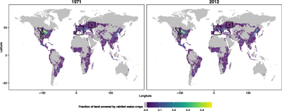
Figure A1. Fraction of land used for non-irrigated maize crops in 1971 and 2012, based on HYDE Hoekstra (1998) and appendix of Fader et al (2010) and MIRCA Portmann (et al 2010). The map also shows the regions of interest discussed insection section 4.2: 1 = Great Plains, 2 = Central Europe, 3 = western Russia.
Download figure:
Standard image High-resolution image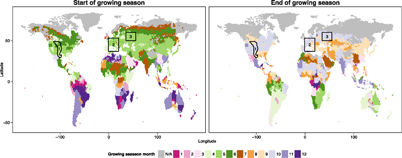
Figure A2. Growing season start end end months (rounded) for non-irrigated maize crops, based on (Sacks et al 2010, Portmann et al 2010 and Elliott et al 2015). The map also shows the regions of interest discussed in section section 4.2: 1 = Great Plains, 2 = Central Europe, 3 = western Russia.
Download figure:
Standard image High-resolution image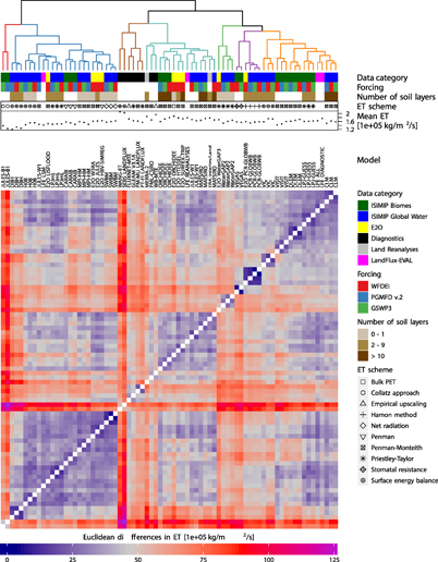
Figure A3. As in figure 2, but based on time-averaged ETtot (Dtavg).
Download figure:
Standard image High-resolution image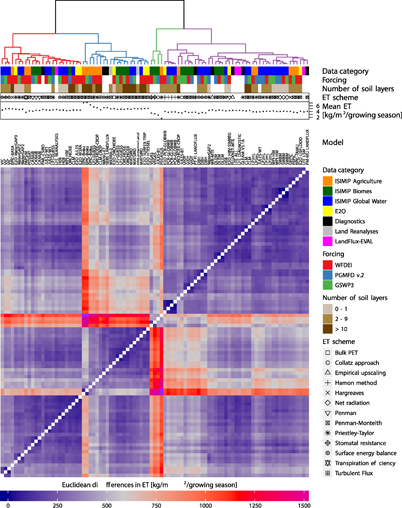
Figure A4. As in figure 3, but based on time-averaged ETmaize (Dtavg).
Download figure:
Standard image High-resolution image
Appendix B. Data preprocessing for comparison with crop model output
In order to perform a cross-sectoral inter-comparison between ETmaize and ETtot, it was necessary to pre-process the original datasets. We first aggregated the monthly estimates (i.e. ETtot) to match the growing season of the non-irrigated maize crops after rounding the respective growing seasons to full months (see figure A2). In a second step, all growing season-specific estimates of ET (i.e. including ET from the crop models) were multiplied by a gridded dataset of time-varying historical cropland patterns which is based on trends of agricultural land from HYDE Hoekstra (1998) and appendix of Fader et al (2010)) and present-day (year 2000) crop and irrigated areas from MIRCA (Portmann et al 2010, see figure A1). By these means, we ensured that an inter-comparisons of ETmaize across all datasets is only performed for grid cells where non-irrigated maize crops are actually growing.
Acknowledgments
This research was funded by the European Research Council DROUGHT-HEAT project (contract 617518). PEGASUS simulations were carried out by D. Deryng on the High Performance Computing Cluster supported by the Research and Specialist Computing Support service at the University of East Anglia. GL was supported by the Office of Science of the US Department of Energy as part of the Integrated Assessment Research Program. CLM water sector simulations were performed using PNNL Institutional Computing at Pacific Northwest National Laboratory. PNNL is operated by Battelle Memorial Institute for the US DOE under contract DE-AC05-76RLO1830. GPW was supported by the Joint DECC and Defra Integrated Climate Program - DECC/Defra (GA01101). J L was supported by the National Natural Science Foundation of China (41625001, 41571022) and partly supported by the Southern University of Science and Technology (Grant no. G01296001).